
Discarding data or dealing with bias?
 based on reviews by 2 anonymous reviewers
Bird population trend analyses for a monitoring scheme with a highly structured sampling design
Abstract
Recommendation: posted 09 April 2025, validated 09 April 2025
Paquet, M. (2025) Discarding data or dealing with bias?. Peer Community in Ecology, 100748. https://doi.org/10.24072/pci.ecology.100748
Recommendation
Obtaining accurate estimates of population trends is crucial to assess populations’ status and make more informed decisions, notably for conservation measures. However, analyzing data we have at hand, including data from systematic monitoring programs, typically induces some bias one way or another (Buckland and Johnston 2017). For example, sampling can be biased towards some types of environments (sometimes historically, before being realized and corrected), and observer identity and experience can vary through time (e.g., an increase in observed experience, if ignored, would cause bias towards positive trends). One way to deal with such biases can be to discard some data, for example, from some overrepresented habitats or from first years surveys to minimize observer bias. However, this may lead to sample sizes becoming too small to detect any trends of interest, especially for surveys with already small temporal resolution (e.g., if time series are too short or with too many missing years).
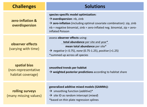
In this study, Rieger et al. (2025) analyzed data from bird surveys from the Ecological Area Sampling in the German federal state North Rhine-Westphalia in order to assess population trends. This survey uses a ‘rolling’ design, meaning that each site is only visited one year within a multi-year rotation (here six), but this allows to cover a high number of sites. To deal with spatial bias, they analyzed trends per natural region. To control for observer effects, they used a correction factor as an explanatory variable (based on the ratio between the total abundance of all species per site per survey year and the mean total abundance on the same site across all survey years). To deal with the fact that count data for some species but not others may be zero inflated and/or over dispersed, they performed species-specific optimization regarding data distribution (and also regarding inclusion of continuous and categorical covariates). Finally, they deal with the many missing values per year per site (due to the rolling design) by using generalized additive mixed models with site identity as a random intercept.
Importantly, the authors assess how accounting for these biases affects estimates (quite strongly so for some species) and study the consistency of the results with trends estimated from the German Common Bird Monitoring scheme using the software TRIM (Pannekoek and van Strien 2001).
I appreciated their cautious interpretation of their results and of the generalizability of their approach to other datasets. I also recommend that the readers read the review history of the preprint (and I take the opportunity to thank the reviewers and the authors again for the very constructive exchange).
References
Buckland, S., and A. Johnston. 2017. Monitoring the biodiversity of regions: Key principles and possible pitfalls. Biological Conservation 214: 23-34. https://doi.org/10.1016/j.biocon.2017.07.034
Pannekoek, J., van Strienand, A. J. 2001. TRIM 3 manual (Trends & Indices for Monitoring Data). CBS Statistics Netherlands, Voorburg, The Netherlands.
Rieger, M. R., Grüneberg, C., Oberhaus, M., Trautmann, S., Parepa, M., Anthes, N., 2025. Bird population trend analyses for a monitoring scheme with a highly structured sampling design. BioRxiv, ver.3 peer-reviewed and recommended by PCI Ecology https://doi.org/10.1101/2024.06.30.601382

The recommender in charge of the evaluation of the article and the reviewers declared that they have no conflict of interest (as defined in the code of conduct of PCI) with the authors or with the content of the article. The authors declared that they comply with the PCI rule of having no financial conflicts of interest in relation to the content of the article.
The development of this workflow has been financially supported by State Agency for Nature, Environment and Climate in North Rhine-Westphalia (LANUK, former LANUV) to University of Tübingen.
Evaluation round #2
DOI or URL of the preprint: https://doi.org/10.1101/2024.06.30.601382
Version of the preprint: 2
Author's Reply, 26 Mar 2025
Decision by Matthieu Paquet, posted 05 Mar 2025, validated 05 Mar 2025
Dear authors,
Your revised manuscript has now been evaluated by the two previous reviewers and they are overall very happy with your revision. Once you have adressed their minor suggestions, I will be happy to recommend your preprint.
In addition please address my following minor comments:
1) When running the code "EAS_bird-v1.1/m-rieger-EAS_bird-f1e6cc6/EAS_bird.R" I get following error message by the end: "There is no final model for 'Black Redstart'"
2) Line 687: change "re_formual = NA" with "re_formula = NA"
3) Lines 800 and 1548: isn't it four, not five, species?
I look forward to receiving your revision,
Matthieu
Reviewed by anonymous reviewer 1, 25 Feb 2025
Most of the concerns with the procedures of the previous versions have been addressed and improved. In general, this is a thoroughly conducted study where a lot of effort have been put into trying to deal with the challenges of the data. While it is not so clear that the components of the analysis are particularly novel (except perhaps for the specifics of the treatment of observer effects), it is an overall nicely worked case study for a fairly complex data set.
L125-129. This suggests that the biogeographic regions are not used which could lead to the question of why you mention them here. You state later how you use them, but would be good to give a hint here.
L146. 2021 should be 2011?
L200. What basis dimension did you use for the smoothers?
L210. Why do you think that landscape type is the main driver of difference in trends? I.e. why does landscape type “account for spatial bias”?
L235. With only 2-4 observations per site, it would be next to impossible to provide a meaningful estimate of autocorrelation.
L244. Should explain that tree depth refers to the Hamiltonian Monte Carlo algorithm in Stan.
L257. What was the computational cost of estimating the models in general, and particularly running the cross validation? Could be useful to know for readers considering an approach like this.
L295. This choice means hat the uncertainty of the index is not an uncertainty of change. In the panels in Fig 6 the uncertainties (blue and yellow) are therefore not comparable, they mean different things.
Fig 5. It seems like more surveys are being flagged as negative compared to positive. Could imbalance of the flagging affect the corrections?
L420-423. It is not just the choice of baseline, the smooth trend does not capture difference in abundance between the first few years and later years.
L471. How do you know it is effective? I.e. that there are not other spatial causes of bias that your model is missing.
L487-492. This begs the question of what the reason for the change in the observer effects may be. You addressed this in the response, but it seems like important information to add here.
https://doi.org/10.24072/pci.ecology.100748.rev21Reviewed by anonymous reviewer 2, 03 Mar 2025
Evaluation round #1
DOI or URL of the preprint: https://doi.org/10.1101/2024.06.30.601382
Version of the preprint: 1
Author's Reply, 13 Feb 2025
Decision by Matthieu Paquet, posted 18 Oct 2024, validated 18 Oct 2024
Dear Authors,
Thank you for submitting your preprint for review at PCI Ecology. Your manuscript entitled “Analysing bird population trends from monitoring data with highly structured sampling designs” has been thoroughly reviewed by two reviewers. While both reviewers highlight the importance and difficulty of dealing with unbalanced sampling when estimating population trends, they both raise several important issues. Notably, both reviewers pointed at the fact that the proposed weighting method artificially increases statistical precision for underrepresented regions (which is briefly acknowledged in the discussion). More generally, since the aim of the manuscript is to provide a new method that better deals with imbalanced sampling, then I concur with the reviewers that 1) the actual efficiency of the method should be better assessed, e.g., using simulations, and 2) this method should be compared directly with existing methods.
You will find their detailed reviews below.
I look forward to reading a revised version of this preprint.
Best wishes,
Matthieu
Reviewed by anonymous reviewer 1, 26 Jul 2024
The paper proposes GAMs combined with weighting as a method for adjusting trend estimation for strong imbalance in population survey data. Unbalanced sampling is a common issue in population surveys and statistical tools and models developed for such data typically deal with unbalanced sampling one way or the other. The TRIM software commonly used for bird surveys in Europe is e.g. designed specifically to address such issues, using a combination of site effects and imputation. Imputation/post-hoc weights (i.e. fitting the model to available data, then weighting model predictions) is probably the most common approach to try to correct for imbalance taken in previous studies.
The authors here instead use a weighted Bayesian likelihood to adjust for imbalance, which in general is an interesting idea. Also, while imbalance has been often discussed and considerable effort is often put into addressing it, I know of few studies that thoroughly investigate strong imbalance in animal survey data. Another interesting idea proposed here is to adjust for survey effort using total counts across species.
Given that the papers is written with a methods focus, I found it somewhat lacking comparisons to previous approaches, particularly regarding the likelihood weights. If the aim of the paper is to provide a method that is better at handling strong imbalance than other methods, which is how I read it, then more effort needs to be put into showing how the approach is better at dealing with imbalance. On the other hand, if the aim was to show how imbalance may be dealt with in the case study, then the “methods” aspects of the paper could be toned down and new material may not be needed (i.e. suggest that this is one way of dealing with imbalance rather than it being a better way).
If the former route is taken, we need to know more about how the suggested methods/models compare to other methods, e.g. imputation methods such as those in TRIM, or perhaps models such as those of Harrison et al 2014 (spatio-temporal GAMs fitted without weights but with predictions over a representative set of points).
Harrison et al. (2014). Assessing trends in biodiversity over space and time using the example of British breeding birds. Journal of Applied Ecology, 51, 1650--1660. https://doi.org/10.1111/1365-2664.12316
The likelihood weights also need to be discussed more. As far as I understand, this weighting is essentially ad-hoc. The weights are constructed to adjust for imbalance, but there is no particular motivation for the resulting weighted likelihood. Intuitively, the weights are cleverly constructed and make a lot of sense in that sites that are in over-represented bioregions get downweighted, as illustrated in Fig. 7. However, the flip side is that surveys in under-represented regions get upweighted. In effect, if I am understanding correcly, abundances at such sites will be treated as if they were multiple independent data points. A site with a weight of 2 would be treated as 2 data points. Thus positive weights artificially inflate precision provided by corresponding data points, which will lead to underestimation of uncertainty from those points. This issue is briefly mentioned in the Discussion, but needs to be made more explicit and more thoroughly discussed. It may have limited effect in this particular study because most weights are small, but as a general principle it seems problematic and hard to justify.
Another issue with the weights is that they cannot adjust for imbalance if data are missing entirely from one of the categories. This is solved here by smoothing over time. However, the meaning of the weights becomes less clear in such a case. The point of the weights was to get data that are balanced among the classes, but since this cannot be done when a class is missing it could be argued that all weights should be zero (this also makes some mathematical sense as the equation on line 151 suggests infinite weights for missing areas).
The above ad-hoc nature of the weights should be stated up-front, not in the least to motivate future work with more rigorous derivation of weighted likelihoods. Alternatively of course, you could provide more rigorous justifications yourselves.
L 44. To me this feels like 6 sources rather than 2.
L79-80. TRIM is indeed widely used in Europe, however, I would not agree that it is the “current analytical standard” (although I’m not sure I correctly understand what this means). E.g. it is not widely used for North American data, and many other types of models have been suggested for this type of data.
L85-86. It is not clear in what sense “TRIM reaches its limits”?
L89-91. Not fully true as TRIM can estimate annual indices and include breakpoints.
L144-147. If the balance of the subsampling was changed, then it cannot be a strict 6-year rolling scheme as suggested in the first paragraph of the methods. This needs clarification.
L149. It is not obvious what “weighted response measures” means. Explain how the weights work. My understanding is that the weights multiply the log-likelihood contribution of each data point.
L195. Need more information about the response. What is “abundance”, is it a count or something else?
L201-204. How was this assessment done, i.e. how did you determine if there were excessive zeroes or overdispersion?
L204. Just 0.5, or also 1.5, 2.5 etc? If so, an alternative is to use 2*abundance as the response with an offset = log(2).
L216-219. The use of weights for natural regions suggests that you believe the trends are not the same, so I don’t follow the argument for only estimating separate curves per bioregion?
L208-227. The model formulation is not crystal clear to me from the text. I found the model formula in the footnote of Table 1 but it felt somewhat tucked away there. I would suggest to display the formula more prominently, perhaps in the main text or at least with a reference in the main text. Also, the main model formula appears not fully correct as survey_year appears both in s() and as a linear term which would be redundant. Perhaps you meant
~ s(survey year, by = R) + R + poly(PC1, 2) + poly(PC2, 2) + poly(PC3, 2) + OE + (1|ID)
so that intercepts can vary among regions as suggested in the documentation for the by argument in ?mgcv::s.
What priors did you use?
L245. Why were these four statistics chosen? I.e. why do you consider them particularly important for estimating population trends from these data?
L247. How did you treat random effects when simulating new data for the p-values? E.g., where site effects regenerated, or did you use their estimated values?
L248-253. Bayesian p-values close to 0 and 1 do flag issues as you suggest, but there’s no reason as far as I know to expect that they have to be close to 0.5 for a good model. This calls the “selection value” into question. Optimizing to get p-values as close as possible to 0.5 could lead to overfitting. The selection value also seems to suggest that one can somehow trade off a single poor p-value with better ones. E.g., if two p-values for one model are 0.01 and 0.5, the selection value would be 0.24. Another model might have the same two p-values both equal to 0.85 and a selection value of 0.25. This would suggest that the first model with the strongest indication of poor fit should be preferred. I also don’t understand how you are using this value and why it is needed. Unless there is some justification for it that I’m missing, I suggest to omit.
L265-267. How were they combined? Were predictions combined at the log scale or at the response scale? If the former, how should we interpret the combined trend estimate in terms of abunance? If the latter, how did you deal with imbalance in covariate values between regions? Explain and motivate the computation.
L269. Notation ab here is slightly confusing (is it a times b, or a single variable ab?). Use a single letter instead (why not N if ab is expected abundance).
L270. For clarity it would be better to refer to the i as posterior draws or posterior samples instead of simulations, if that’s what you mean.
L281. I don’t see why you’d want to use the posterior mean in the denominator. I would rather have expected you compute the posterior distribution of the index, i.e. make posterior inference for abij/abiJ, just as you seem to have done for the differences on L269. The uncertainty of the index would then be 0 in 2006 as expected, similarly to e.g. TRIM indices.
L293-295. How does the MhB match temporally to the EAS which was collected during a long period from February to July?
L299-301. I can’t follow the sentence, rephrase?
L304-305. This ‘coincidence’ will be large if there is large uncertainty in the EAS estimates. They could also be very different from the ‘coincidence’ computed by reversing the roles of the two estimates (i.e. the fraction of EAS estimates within 95% Mhb intervals). Would be good with an explanation of what it is supposed to measure.
L320-324. More details about the model comparisons are need: How did you “optimise models”? What does “best-performing model” and “comparably good performance” mean? From the Table caption you seem to be using 0.3 and 0.7 as cutoffs for “good performance”, was there any rationale behind this choice? Why do you need to determine a “best-performing model” when you are going forward with the most parsimonious model with “good performance”? How do you determine which model is “most parsimonious”?
L338. Since you include a random site effects, your model should be able to capture among-site overdispersion even with a Poisson response. The NB might rather account for overdispersion among years since the model can only capture smooth inter-annual variation (there are no random year effects as I understood it). Or it might pick up overdispersion in the interaction between year and site.
L365. I’m not sure what the Poisson histograms in Fig 3 represent, do they just show the Poisson distribution with mean equal to the overall mean of the data? If so I don’t see the point of including it as this distribution says little about whether the Poisson is a reasonable response for the model (i.e. with covariates, random effects etc histograms could look very different even if the response was Poisson).
L382-388. It would be interesting to see how this would compare to trends derived using the unweighted model for prediction and then weighting the predictions, i.e. post-hoc weighting. Would also be interesting to see how it compares to other approaches, as I suggested above.
L390-. This is interesting. Do you have any explanation for these strong effects? Is it just a question of observer experience. If so, why are they so large? Could there be other explanations?
L409-411. It is hard to interpret this result at present because the CIs of the EAS do not measure uncertainty of the relative index, see previous comment.
L412. You could reduce this sensitivity by using the mean across the full time period as the baseline (if you have access to the MhB data), instead of using a single year.
L414-415. While the trends in Fig 7b are consistent in their general shape, they suggest very different magnitudes of change. Something that the correlation misses. In other words, you could have perfectly correlated indices that show entirely different magnitudes of change, which may be worth pointing out. Also, you could consider complementing the two measures with something that measures the difference in values between the two indices, maybe something based on the differences between log-transformed indices.
L483. To strictly evaluate bias one needs to know the truth which we don’t here. If you mean that inclusion of observer effects reduced the trends, or that trends came closer to MhB, then say so instead.
L492. Not sure what flagging of extreme years you are referring to, or how that would counter the effects discussed here.
L493-496. This can also go the other way. Some species are easy to detect and counts may not be strongly linked to observer skill. The correction could bias trends for such species.
L507. What covariates do you mean?
https://doi.org/10.24072/pci.ecology.100748.rev11