
Gene flow in the city. Unravelling the mechanisms behind the variability in urbanization effects on genetic patterns.
 based on reviews by 2 anonymous reviewers
How does dispersal shape the genetic patterns of animal populations in European cities? A simulation approach
Abstract
Recommendation: posted 19 March 2024, validated 19 March 2024
Coulon, A. (2024) Gene flow in the city. Unravelling the mechanisms behind the variability in urbanization effects on genetic patterns.. Peer Community in Ecology, 100579. https://doi.org/10.24072/pci.ecology.100579
Recommendation
Worldwide, city expansion is happening at a fast rate and at the same time, urbanists are more and more required to make place for biodiversity. Choices have to be made regarding the area and spatial arrangement of suitable spaces for non-human living organisms, that will favor the long-term survival of their populations. To guide those choices, it is necessary to understand the mechanisms driving the effects of land management on biodiversity.
Research results on the effects of urbanization on genetic diversity have been very diverse, with studies showing higher genetic diversity in rural than in urban populations (e.g. Delaney et al. 2010), the contrary (e.g. Miles et al. 2018) or no difference (e.g. Schoville et al. 2013). The same is true for studies investigating genetic differentiation. The reasons for these differences probably lie in the relative intensities of gene flow and genetic drift in each case study, which are hard to disentangle and quantify in empirical datasets.
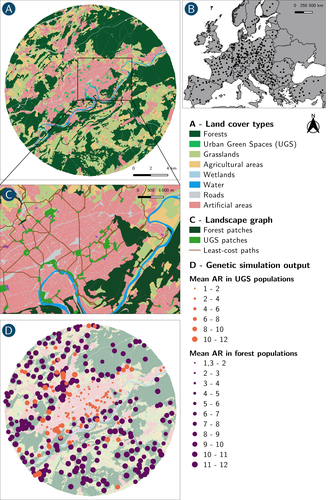
In their paper, Savary et al. (2024) used an elegant and powerful simulation approach to better understand the diversity of observed patterns and investigate the effects of dispersal limitation on genetic patterns (diversity and differentiation). Their simulations involved the landscapes of 325 real European cities, each under three different scenarios mimicking 3 virtual urban tolerant species with different abilities to move within cities while genetic drift intensity was held constant across scenarios. The cities were chosen so that the proportion of artificial areas was held constant (20%) but their location and shape varied. This design allowed the authors to investigate the effect of connectivity and spatial configuration of habitat on the genetic responses to spatial variations in dispersal in cities.
The main results of this simulation study demonstrate that variations in dispersal spatial patterns, for a given level of genetic drift, trigger variations in genetic patterns. Genetic diversity was lower and genetic differentiation was larger when species had more difficulties to move through the more hostile components of the urban environment. The increase of the relative importance of drift over gene flow when dispersal was spatially more constrained was visible through the associated disappearance of the pattern of isolation by resistance. Forest patches (usually located at the periphery of the cities) usually exhibited larger genetic diversity and were less differentiated than urban green spaces. But interestingly, the presence of habitat patches at the interface between forest and urban green spaces lowered those differences through the promotion of gene flow.
One other noticeable result, from a landscape genetic method point of view, is the fact that there might be a limit to the detection of barriers to genetic clusters through clustering analyses because of the increased relative effect of genetic drift. This result needs to be confirmed, though, as genetic structure has only been investigated with a recent approach based on spatial graphs. It would be interesting to also analyze those results with the usual Bayesian genetic clustering approaches.
Overall, this study addresses an important scientific question about the mechanisms explaining the diversity of observed genetic patterns in cities. But it also provides timely cues for connectivity conservation and restoration applied to cities.
References
Delaney, K. S., Riley, S. P., and Fisher, R. N. (2010). A rapid, strong, and convergent genetic response to urban habitat fragmentation in four divergent and widespread vertebrates. PLoS ONE, 5(9):e12767.
https://doi.org/10.1371/journal.pone.0012767
Miles, L. S., Dyer, R. J., and Verrelli, B. C. (2018). Urban hubs of connectivity: Contrasting patterns of gene flow within and among cities in the western black widow spider. Proceedings of the Royal Society B, 285(1884):20181224. https://doi.org/10.1098/rspb.2018.1224
Savary P., Tannier C., Foltête J.-C., Bourgeois M., Vuidel G., Khimoun A., Moal H., and Garnier S. (2024). How does dispersal shape the genetic patterns of animal populations in European cities? A simulation approach. EcoEvoRxiv, ver. 3 peer-reviewed and recommended by Peer Community in Ecology. https://doi.org/10.32942/X2JS41.
Schoville, S. D., Widmer, I., Deschamps-Cottin, M., and Manel, S. (2013). Morphological clines and weak drift along an urbanization gradient in the butterfly, Pieris rapae. PLoS ONE, 8(12):e83095.
https://doi.org/10.1371/journal.pone.0083095

The recommender in charge of the evaluation of the article and the reviewers declared that they have no conflict of interest (as defined in the code of conduct of PCI) with the authors or with the content of the article. The authors declared that they comply with the PCI rule of having no financial conflicts of interest in relation to the content of the article.
The authors declare that they have received no specific funding for this study
Evaluation round #2
DOI or URL of the preprint: https://doi.org/10.32942/X2JS41
Version of the preprint: 2
Author's Reply, 18 Mar 2024
Dear Dr. Coulon,
We would like to thank you for your thorough evaluation of our manuscript and for this opportunity to further improve its clarity. We diligently addressed your two comments and provide below a detailed response to each of them. The main text and corresponding preprint have been updated accordingly. We are also attaching a revised version of our manuscript with tracked changes.
Sincerely,
Paul Savary, on behalf of my co-authors
Comment 1: l.206-207, "the length in metric units of the least-cost paths not crossing the most unfavorable areas": what does "the most unfavorable areas" exactly means? Artificial areas? Artificial areas + roads + water? How did you proceed, did you subsample the LCPs that did not cross those land cover categories?
RESPONSE: We thank you for the opportunity to clarify this complex step of our analytical workflow. We rephrased this section to better explain how we converted a distance of 5 km into cost units (lines 205-212). We used a specific functionality of the Graphab software program allowing users to restrain the computed least-cost paths to those that do not cross pixels having large cost values. To clarify our explanation without entering into technical details, we splitted it in several sentences while recalling what the least favorable areas were, under our modelling assumptions (as per your comment). We also replaced the term "most unfavorable" by "least favorable" for the sake of coherence in the terminology used. This section now reads as:
"To obtain d_5km, we assessed the relationship between (1) the length in metric units of the least-cost paths not crossing the least favorable areas and (2) the corresponding cost-distances, using log-log linear regressions (Tournant et al., 2013). For that purpose, we only considered the set of paths (spatial trajectories and associated cost-distances) that never crossed any pixel of artificial area, road or water, as they are supposed to be representative of the most common species movements. We then used the estimated relationship between the length of these paths and their cost-distances to convert 5 km into cost units and computed the average converted value for each urban area and each scenario."
Comment 2: IBLR analyses, l.299-303: The explanation of the interpretation of the DMC values is a bit confusing. Indeed, you say that "large values are supposed to indicate cases where IBLR leads to a continuous and linear relationship (...)", but what do you exactly mean by "large"? The standardized DMC is supposed to range between 0 and 1, but then, l.302 you say that "on the contrary, values between 0 and 1 could indicate the presence of a plateau (...)". I don't understand what the large DMC values indicating a linear relationship can be, then.
RESPONSE: We thank you for noticing this source of confusion in our explanation. As you relevantly pointed out, strictly speaking, only a DMC value of 1 indicates that a continuous linear IBD relationship is observed at the scale of the whole study area, whereas values ranging from 0 to 1 tend to indicate that this relationship exhibits a plateau at intermediate spatial scales. We therefore corrected this sentence by replacing "Large values" with "A value of 1" (lines 302-303).
Decision by Aurélie Coulon, posted 15 Mar 2024, validated 15 Mar 2024
Dear authors,
I have read your revised preprint and your answers to the reviewers’ comments. I think you have adequately addressed all of them, and that your ms is almost ready for recommendation. I only ask you to address the two minor points below. In the meantime, I will be preparing my recommendation.
Best,
Aurélie Coulon.
l.206-207, “the length in metric units of the least-cost paths not crossing the most unfavorable areas”: what does “the most unfavorable areas” exactly means? Artificial areas? Artificial areas + roads + water? How did you proceed, did you subsample the LCPs that did not cross those land cover categories?
IBLR analyses, l.299-303: The explanation of the interpretation of the DMC values is a bit confusing. Indeed, you say that “large values are supposed to indicate cases where IBLR leads to a continuous and linear relationship (…)”, but what do you exactly mean by “large”? The standardized DMC is supposed to range between 0 and 1, but then, l.302 you say that “on the contrary, values between 0 and 1 could indicate the presence of a plateau (…)”. I don’t understand what the large DMC values indicating a linear relationship can be, then.
Evaluation round #1
DOI or URL of the preprint: https://doi.org/10.32942/X2JS41
Version of the preprint: 1
Author's Reply, 06 Mar 2024
Dear Dr. Coulon,
Please find attached our response letter and a revised version of our manuscript with tracked changes.
Note that the revised version of the preprint is available on EcoEvoRxiv: https://doi.org/https://doi.org/10.32942/X2JS41
We have also updated the supporting information: https://doi.org/10.5281/zenodo.10789195
This link is included in the revised version of the manuscript.
Best regards,
The Authors
Decision by Aurélie Coulon, posted 09 Jan 2024, validated 09 Jan 2024
Dear Dr Savary and collaborators,
After unexpected difficulties to secure reviews, I have finally received two reports on your preprint entitled “How does dispersal shape the genetic structure of animal populations in European cities? A simulation approach”. I sincerely apologize for the unusual long time that was necessary before getting back to you about this preprint.
Both reviewers are enthusiastic about your manuscript. I agree with them that overall, it presents a very interesting and stimulating study and that it is nicely written. The two reviewers highlighted a few limitations in your simulations that need at least to be discussed in details. They also made a number of suggestions of improvements in the writing that I suggest you follow.
I will be happy to read the new version of your manuscript and assess it for recommendation.
Best,
Aurélie Coulon.
Reviewed by anonymous reviewer 2, 19 Oct 2023
General comments:
The paper presents a very interesting and original simulation-based investigation of the effect of the permeability of urban environments (i.e. dispersal limitation) on neutral genetic patterns in populations of urban tolerant species, using the example of forest species occupying both forest and urban green spaces (UGS). Authors simulated genetic data across a set of 325 cities in Europe. Disentangling the influence of drift and gene flow (/dispersal) on genetic patterns is one of the biggest challenges in landscape genetics. Simulation studies are useful to produce predictions and investigate the effect of these processes on observed genetic patterns (genetic diversity and genetic structure). In this context, the present paper is a nice and original contribution in the specific context of urban ecology. I found the study well designed, relevant and timely. The paper is well written and easy to get through. I have though a few suggestions to improve it (see specific comments). Overall, I find the methods convincing and the reported findings interesting. My suggestion is to accept the paper with minor modifications.
Simulation studies in landscape genetics are generally based on simulated landscapes. Using real landscapes is an originality of the paper. The number of selected cities (N = 325) is large enough to allow authors to draw general conclusions. However, I wonder why the authors choose to base the study on real cities rather than simulating urban landscapes (and controlling their topology). I feel it might have been a more simple approach to address the research objective (in addition, the process to select cities is not totally clear to me, see specific comment below). Controlling parameters would have allowed to test some predictions. I do not recommend to re-run analyses with simulated urban landscapes but it will be interesting to explain and discuss this choice in the paper.
In general, there was a lack of descriptive information of the data. For example, it would be interesting to present metrics describing raw differences between forested and UGS patches (location, average size, …). I wonder if the results from genetic simulations do not simply reflect these differences (plus the differences in habitat connectivity that were nicely summarized with the F and EC metrics). Actually, parameters of the genetic simulations are identical for forested and UGS patches (same dispersal cost value, no differences in “carrying capacity” or in dispersal rates). Genetic simulations results could have been analyzed without contrasting these two habitats. In fact, this distinction just summarizes differences in size, location and connectivity between the two habitat types. I wonder if genetic response modelling would have been more informative by directly using such continuous metrics in the genetic response modelling (at least location and connectivity such as the Flux connectivity metric).
Replicates of genetic simulations. Regarding genetic simulations, it seems that there was only one simulation per city and scenario. I wonder if it would be possible to investigate the sensitivity of results to initial conditions in each city x scenario simulation (in particular populations sizes and their location, given that not all habitats patches are occupied). Running e.g. 5 or 10 simulations per city would probably lead more consistent results. Although I don’t really measure the amount of computing time this would take (10x3x325= almost 10,000 simulations). You might at least explore and quantify this variability on a few cities (eg with contrasted number of habitat patches).
Statistical modelling. I liked the use of statistical modelling to summarize the simulations results for genetic metrics. Regarding the genetic differentiation metric, the response variable is a paired genetic distance. I do not think this is appropriate to run LM/GLM/GLMMM on this type of data as they are not independent (a single population is involved in multiple pairs). Permutation tests should be more appropriate in that case. However, since you do not interpret the P values I think this should not be considered as a too serious problem.
Specific comments:
Title : “Genetic pattern” might be better than “genetic structure” as you explored both genetic diversity and genetic structure.
L22-23: this is only because of simulation parameters that reflected size difference between forest and UGS patches. You should focus on the interaction with scenario.
L58 : « neutral genetic markers are also affected by urbanization » I see what you mean, and agree, however, I found it a bit clumsy. Please reformulate. Eg « neutral genetic patterns…»
L69 : This section seems to provide general background on processes acting on genetic patterns, while the following section focuses on urban tolerant species. Thus, I would not start with a sentence specifying “in these urban tolerant species” as everything following in the section is general and apply to all species (same for “urban populations” L75).
L85-87: I suggest to move this sentence (which is very important) to the previous section.
L94-97: The idea is not clear, I suggest to remove the sentence (or reformulate).
L108 : could you please be more specific on the « potential factors » ?
L116-120: I suggest to move this section to the introduction. Would be nice at the end of the 4th section.
L122 : change to «… forest species occupying both forest and UGS »
L135-136: It would be interesting to somehow quantify this differential distribution of forest and UGS patches in cities (e.g. kind of density plot with distance from city center for each type and / or of their relative proportion).
L139-140: I think a single reference could be enough here.
L148-156: I found the method of cities and radius size selection complex and its description was unclear. Did you first set up a minimal/maximal radius? Did you increase radius step by step (size of steps?), until having a proportion of artificial area at 20%? Besides, the sensitivity analysis on radius size in the supporting information is useful and convincing.
L158-159: I suggest to remove the first sentence.
L159: these responses -> ‘genetic responses’ or ‘neutral genetic patterns’
L196: The Flux connectivity metric was only calculated to identify “Forest interfaces” and “UGS interfaces” used in the genetic response modelling. I suggest to move this section to the supporting information in order to reduce the length of M&M. It would also be nice to present the distribution of Flux values with a supplementary Figure.
L231-232: first sentence is not necessary to me.
L233: it is also unlikely that all habitat patches are occupied in real metapopulations.
L238-239: This sentence is a bit misleading. Do you mean that you sampled patches to populate them with populations? Did you consider patch size? I guess it is more likely that larger patches are occupied by a population.
L240-242: Could you provide the average size of forested and UGS patches? (maybe better in the “land cover data” section?)
L251: remove “each” (typo?), “on average” sounds better.
L256: did the simulation process allowed the colonization of empty patches?
L251-255: Could you indicate the proportion of habitat patches (per type, forested and UGS) that are occupied? And its variation across cities? Do you think this parameter could affect simulations results (regarding contrasts among scenarios)?
L259: did you test the sensitivity of simulations to the number of generations? Did genetic simulations reach an equilibrium after 250 generations?
L265: not clear. To keep the total population or the local population constant?
L287-288: Sentence not necessary. I suggest to remove.
L294-295: It might be more clear to indicate that it correspond to a ratio of the maximal DMC value possible for a given city, thus varying from 0 to 1.
L330: genetic structure -> genetic pattern (unless you think it only affected genetic structure?)
L339-340: I did not get the point. I agree that you controlled population sizes (according to patch size which are different between Forest and UGS) and dispersal cost values associated with scenarios, so you expect significant p-values related to these factors. However, models should be useful to test the interaction between scenarios and habitat type/type of pair.
L343-344: “When…” I first understood that habitat type/type of pair and cost scenario were included in all models (and so the interaction). Please explain. Also, why don’t you show and discuss the estimate of the interaction and its p-value? It could give stronger support to your main conclusions.
L356: please provide at least the range or maybe more details on the distribution of radius sizes in the dataset (in supplementary data). Is there a strong correlation between radius size and population (inhabitants) size?
L377: very high -> higher
L378-379: I don’t understand how did you get a separate estimate for forest and UGS interfaces. It is not clear in the methods and results sections. did you include interface as a fixed effect? Ran a separate model? The “genetic response modelling” section needs to be improved with more details.
I found the “sensitivity” analysis very interesting and convincing. Did you consider running models with Radius area or total habitat area as covariates?
L447: “dispersal behavior” Not sure about the use of this term. It reflects both dispersal rate (set constant in the simulations) and dispersal distance. In simulations you only explored distance through the modulation of matrix resistance / permeability. You should be more specific.
L448-449:
L518-524: I suggest to remove this section.
L525: To assess the spatial distribution of urban habitat types it could be interesting to include distance from city center in genetic response modelling analyses (at least in models for genetic diversity).
Fig 1: I unsuccessfully tried to figure out which city is shown in the example. Not sure this information is important to improve the quality of the MS but I still like to know the answer :)
https://doi.org/10.24072/pci.ecology.100579.rev11
Reviewed by anonymous reviewer 1, 05 Jan 2024
The reviewed manuscript, “How does dispersal shape the genetic structure of animal populations in European cities? A simulation approach”, seeks to understand the role of gene flow and broad-scale landscape effects on the genetic outcomes and population trajectories of urban tolerant wildlife species. The authors present an impressively large simulation study, which differs from many theoretical landscape genetic studies by using empirical spatial data representing 325 cities across Europe on which they seeded random genetic variation and simulated migration patterns across three cost scenarios. The analyses provide important insights into the relative role of gene flow vs. genetic drift and provide actionable advice for the conservation management of urban wildlife populations. The writing, methodology, and results are all of very high quality with few major issues.
Important issues:
Two important simplifications were used within the presented analyses, which may have biased analyses. First, landcover classes were grouped and simplified, treating all types of built urban areas as “artificial areas”, including low and very low density urban fabric. While urban wildlife may prefer dispersing through continuous green spaces (forest or UGS), built urban areas likely provide supplementary dispersal pathways that are ignored in this analysis. Considering the wide-reaching interpretation about the permeability of urban landscapes, I would like to see results for cost scenarios in which the built environment is treated in a more nuanced way, perhaps with artificial areas broken up into moderate and high cost areas (e.g. with low-density areas given a moderate cost) rather than the entire built environment treated uniformly as high cost. While the “Limitations” section does mention the lack of detail here, citing the need for finer-grained resolution data ignores the presence of additional detail within current spatial data that was ignored through study design. Second, the focus on dispersal via the shortest or least cost path simplifies the simulated dispersal behavior and reduces the importance of patch pairs that may have multiple similar dispersal routes. Circuit-theory approaches would better account for the presence of these more diffuse dispersal networks. I don’t necessarily think that these simplifications negate or discount the presented results, but I would like to see more discussion of these aspects in the discussion section.
Given the use of true urban landscapes within the simulations, the authors are in a position to provide valuable resource to municipal and national institutions seeking to improve wildlife connectivity. If possible, the authors should seek to provide maps or quantitative descriptions of important habitat patches or dispersal routes/barriers at the individual city level. At a minimum, an offer should be made in the discussion to provide this information through private correspondence.
Minor issues noted:
L20: the claim that simulations “reproduced empirically observed results” is not supported with quantitative analysis, so this phrase is misleading. The discussion provides extremely brief claims that outcomes mirrored several cited publications but provides no visual or quantitative comparison for the audience. Either include more explicit comparisons in the text, or soften this language.
L44: “timely needed” …missing comma or remove one word.
L73: populations must not be “well connected” to facilitate genetic exchange. Moderately or even poorly connected populations can allow gene flow, and only minor levels of gene flow are needed to prevent allelic dropout or intense differentiation.
L77: considering the citation of specific gene flow/drift scenarios from Hutchison & Templeton in the discussion, a more in-depth description of the theoretical expectations noted here is warranted.
L82: double closed parentheses
L90: define UGS in this first use of the acronym in main text
L122: “forest species”… should this be “forest-dwellling”
L130: define OECD
L136: given the importance of UGS vs Forest patches throughout the study, a more detailed description of UGS is warranted. Are there canopy cover cutoffs that would make an interior patch into a “forest”. Are there more detailed descriptions of the habitat available?
L145: “led differences” edited to “led to differences”
L266: “for every 20 loci”, does this indicate that there are a total of 20 loci. It is unclear how many loci are being simulated.
L377: provide examples of what is meant by “high” and “very high” allelic richness, particularly in relation to the starting genetic diversity.
L472: the claim that the individuals “range” does not change seems inaccurate. IF the total endured cost stayed the same but the cost per cell increased, then the “geographic range” of the dispersers would decrease. Perhaps clarification on what is meant by “range” is warranted here or earlier in the text.
L478-485: comparisons to empirical data are extremely simplified and provide little detail. I would like to see more explicit descriptions of the species involved, the empirical landscape being compared to, and the findings of those papers. The citation of only two empirical studies is underwhelming given claims made in the abstract.
https://doi.org/10.24072/pci.ecology.100579.rev12