Spatial patterns and autocorrelation challenges in ecological conservation

Eric Goberville

doi:10.24072/pci.ecology.100536

Back

Recommendation

Share Tweet

Printable page

Spatial patterns and autocorrelation challenges in ecological conservation

Eric Goberville based on reviews by Nigel Yoccoz and Charles J Marsh

A recommendation of:

Efficient sampling designs to assess biodiversity spatial autocorrelation : should we go fractal?

Fabien Laroche (2023), bioRxiv, ver.4, peer-reviewed and recommended by PCI Ecology https://doi.org/10.1101/2022.07.29.501974

Read preprint in preprint server

Codes used in this study

Scripts used to obtain or analyze results

Abstract

ZH-CN

Submission: posted 21 April 2023, validated 24 April 2023
Recommendation: posted 02 January 2024, validated 03 January 2024

Cite this recommendation as:
Goberville, E. (2024) Spatial patterns and autocorrelation challenges in ecological conservation. Peer Community in Ecology, 100536. 10.24072/pci.ecology.100536

Recommendation

“Pattern, like beauty, is to some extent in the eye of the beholder” (Grant 1977 in Wiens, 1989)

Ecologists are immersed in unraveling the complex spatial patterns that govern species diversity, driven by both practical and theoretical imperatives (Rahbek, 2005; Wang et al., 2019). This dual focus necessitates a practical imperative for strategic biodiversity conservation, requiring a nuanced understanding of locations with peak species richness and dynamic shifts in species assemblages (Chase et al., 2020). Simultaneously, there is a theoretical interest in using diversity patterns as empirical testing grounds for theories explaining factors influencing diversity disparities and the associated increase in species turnover correlated with inter-site distance (Condit et al., 2002).

McGill (2010), in his paper "Matters of Scale", highlights the scale-dependent nature of ecology, aligning with the recognition that spatial autocorrelation is inherent in biogeographical data and often correlated with sample size (Rahbek, 2005). Spatial autocorrelation, often underestimated in ecological studies (Dormann, 2007), occurs when proximate locations exhibit similarities in ecological attributes (Tobler, 1970; Getis, 2010), introducing a latent bias that compromises the robustness of ecological findings (Dormann, 2007; Dormann et al., 2007). This phenomenon serves as both an asset, providing valuable information for inferring processes from patterns (Palma et al. 1999), and a challenge, imposing limitations on hypothesis testing and prediction (Dormann et al., 2007 and references therein). Various factors contribute to spatial autocorrelation, with three primary contributors (Dormann et al., 2007; Legendre, 1993; Legendre and Fortin, 1989; Legendre and Legendre, 2012): (i) distance-related effects in biological processes, (ii) misrepresentation of non-linear relationships between the environment and species as linear and (iii) the oversight of a crucial spatially structured environmental determinant in the statistical model, leading to spatial structuring in the response (Dormann et al., 2007).

Recognising the pivotal role of spatial heterogeneity in ecological theories (Wang et al., 2019), it becomes imperative to discern and address the limitations introduced by spatial autocorrelation (Legendre, 1993). McGill (2011) emphasises that the ultimate goal of biodiversity pattern studies should be to develop a quantitative predictive theory useful for conservation. The spatial dimension's importance in study planning, determining the system's scale, appropriate quadrat size, and spacing between sampling stations, is paramount (Fortin, 1999a,b). Responses to these considerations are intricately linked with study objectives and insights from pre-sampling campaigns, underscoring the need for a nuanced and rigorous approach (Delmelle, 2021).

Understanding statistical techniques and nested sampling designs is crucial to answering fundamental ecological questions (Dormann et al., 2007; McDonald, 2012). In addressing spatial autocorrelation challenges, ecologists must recognize the limitations of many standard statistical methods in ecological studies (Dale and Fortin, 2002; Legendre and Fortin, 1989; Steel et al., 2013). In the initial phases of description or hypothesis generation, ecologists should proactively acknowledge the spatial structure in their data and conduct tests for spatial autocorrelation (for a comprehensive description, see Legendre and Fortin, 1989): various tools, including correlograms, spectral analysis, the Mantel test, and clustering methods, facilitate the assessment and description of spatial structures. The partial Mantel test enables the study of causal models with space as an explanatory variable. Techniques for mapping ecological variables, such as interpolation, trend surface analysis, and constrained clustering, yield maps providing valuable insights into the spatial dynamics of ecological systems.

This refined consideration of spatial autocorrelation emerges as an imperative in ecological research, fostering a deeper and more precise understanding of the intricate interplay between species diversity, spatial patterns, and the inherent limitations imposed by spatial autocorrelation (Legendre et al., 2002). This not only contributes significantly to the scientific discourse in ecology but also aligns with McGill's vision of developing predictive theories for effective conservation (Bacaro et al., 2016; McGill, 2011).

In this study by Fabien Laroche (2023), titled “Efficient sampling designs to assess biodiversity spatial autocorrelation: should we go fractal?” the primary focus was on addressing the challenges associated with estimating the autocorrelation range of species distribution across spatial scales. The study aimed to explore alternative sampling designs, with a particular focus on the application of fractal designs—self-similar designs with well-identified scales. The overarching goal was to evaluate whether fractal designs could offer a more efficient compromise compared to traditional hybrid designs, which involve mixing random sampling points with a systematic grid.

Virtual ecology provides a way to test whether sampling designs can accurately detect or quantify effects of interest before implementing them in the field. Beyond the question of assessing the power of empirical designs, a virtual ecology analysis contributes to clearly formulating the set of questions associated with a design. However, only a few virtual studies have focused on efficient designs to accurately estimate the autocorrelation range of biodiversity variables. In this study, the statistical framework of optimal design of experiments was employed—a methodology often used in building and comparing designs of temporal or spatiotemporal biodiversity surveys but rarely applied to the specific problem of quantifying spatial autocorrelation.

Key findings from the study shed light on optimal sampling strategies, with a notable dependence on the feasible grid mesh size over the study area in relation to expected autocorrelation range values. The results demonstrated that the efficiency of designs varied based on the specific effect under study. Fractal designs, however, exhibited superior performance, particularly when assessing the effect of a monotonic environmental gradient across space.

In conclusion, the study provides valuable insights into the potential benefits of incorporating fractal designs in biodiversity studies, offering a nuanced and efficient approach to estimate spatial autocorrelation. These findings contribute significantly to the ongoing scientific discourse in ecology, providing practical considerations for improving sampling designs in biodiversity assessments.

References

Bacaro, G., Altobelli, A., Cameletti, M., Ciccarelli, D., Martellos, S., Palmer, M.W., Ricotta, C., Rocchini, D., Scheiner, S.M., Tordoni, E., Chiarucci, A., 2016. Incorporating spatial autocorrelation in rarefaction methods: Implications for ecologists and conservation biologists. Ecological Indicators 69, 233-238. https://doi.org/10.1016/j.ecolind.2016.04.026

Chase, J.M., Jeliazkov, A., Ladouceur, E., Viana, D.S., 2020. Biodiversity conservation through the lens of metacommunity ecology. Annals of the New York Academy of Sciences 1469, 86-104. https://doi.org/10.1111/nyas.14378

Condit, R., Pitman, N., Leigh, E.G., Chave, J., Terborgh, J., Foster, R.B., Núñez, P., Aguilar, S., Valencia, R., Villa, G., Muller-Landau, H.C., Losos, E., Hubbell, S.P., 2002. Beta-Diversity in Tropical Forest Trees. Science 295, 666-669. https://doi.org/10.1126/science.1066854

Dale, M.R.T., Fortin, M.-J., 2002. Spatial autocorrelation and statistical tests in ecology. Écoscience 9, 162-167. https://doi.org/10.1080/11956860.2002.11682702

Delmelle, E.M., 2021. Spatial Sampling, in: Fischer, M.M., Nijkamp, P. (Eds.), Handbook of Regional Science. Springer Berlin Heidelberg, Berlin, Heidelberg, pp. 1829-1844.

Dormann, C.F., 2007. Effects of incorporating spatial autocorrelation into the analysis of species distribution data. Global Ecology & Biogeography 16, 129-128. https://doi.org/10.1111/j.1466-8238.2006.00279.x

Dormann, C.F., McPherson, J.M., Araújo, M.B., Bivand, R., Bolliger, J., Carl, G., Davies, R.G., Hirzel, A., Jetz, W., Kissling, W.D., Kühn, I., Ohlemüler, R., Peres-Neto, P.R., Reineking, B., Schröder, B., Schurr, F.M., Wilson, R., 2007. Methods to account for spatial autocorrelation in the analysis of species distributional data: a review. Ecography 33, 609-628. https://doi.org/10.1111/j.2007.0906-7590.05171.x

Fortin, M.-J., 1999a. Effects of quadrat size and data measurement on the detection of boundaries. Journal of Vegetation Science 10, 43-50. https://doi.org/10.2307/3237159

Fortin, M.-J., 1999b. Effects of sampling unit resolution on the estimation of spatial autocorrelation. Écoscience 6, 636-641. https://doi.org/10.1080/11956860.1999.11682547

Getis, A., 2010. Spatial Autocorrelation, in: Fischer, M.M., Getis, A. (Eds.), Handbook of Applied Spatial Analysis: Software Tools, Methods and Applications. Springer Berlin Heidelberg, Berlin, Heidelberg, pp. 255-278.

Laroche, F., 2023. Efficient sampling designs to assess biodiversity spatial autocorrelation: should we go fractal? bioRxiv, 2022.07.29.501974, ver. 4 peer-reviewed and recommended by Peer Community in Ecology. https://doi.org/10.1101/2022.07.29.501974

Legendre, P., 1993. Spatial Autocorrelation: Trouble or New Paradigm? Ecology 74, 1659-1673. https://doi.org/10.2307/1939924

Legendre, P., Dale, M.R.T., Fortin, M.-J., Gurevitch, J., Hohn, M., Myers, D., 2002. The consequences of spatial structure for the design and analysis of ecological field surveys. Ecography 25, 601-615. https://doi.org/10.1034/j.1600-0587.2002.250508.x

Legendre, P., Fortin, M.J., 1989. Spatial pattern and ecological analysis. Vegetatio 80, 107-138. https://doi.org/10.1007/BF00048036

Legendre, P., Legendre, L., 2012. Numerical Ecology, Third Edition ed. Elsevier, The Netherlands.

McDonald, T., 2012. Spatial sampling designs for long-term ecological monitoring, in: Cooper, A.B., Gitzen, R.A., Licht, D.S., Millspaugh, J.J. (Eds.), Design and Analysis of Long-term Ecological Monitoring Studies. Cambridge University Press, Cambridge, pp. 101-125.

McGill, B.J., 2010. Matters of Scale. Science 328, 575-576. https://doi.org/10.1126/science.1188528

McGill, B.J., 2011. Linking biodiversity patterns by autocorrelated random sampling. American Journal of Botany 98, 481-502. https://doi.org/10.3732/ajb.1000509

Rahbek, C., 2005. The role of spatial scale and the perception of large-scale species-richness patterns. Ecology Letters 8, 224-239. https://doi.org/10.1111/j.1461-0248.2004.00701.x

Steel, E.A., Kennedy, M.C., Cunningham, P.G., Stanovick, J.S., 2013. Applied statistics in ecology: common pitfalls and simple solutions. Ecosphere 4, art115. https://doi.org/10.1890/ES13-00160.1

Tobler, W.R., 1970. A Computer Movie Simulating Urban Growth in the Detroit Region. Economic Geography 46, 234-240. https://doi.org/10.2307/143141

Wang, S., Lamy, T., Hallett, L.M., Loreau, M., 2019. Stability and synchrony across ecological hierarchies in heterogeneous metacommunities: linking theory to data. Ecography 42, 1200-1211. https://doi.org/10.1111/ecog.04290

Wiens, J.A., 1989. The ecology of bird communities. Cambridge University Press.

Conflict of interest:
The recommender in charge of the evaluation of the article and the reviewers declared that they have no conflict of interest (as defined in the code of conduct of PCI) with the authors or with the content of the article. The authors declared that they comply with the PCI rule of having no financial conflicts of interest in relation to the content of the article.

Funding:
Agence Nationale de la Recherche (ANR), grant n° 19-CE32-0002-01

Reviews

Toggle reviews

Evaluation round #2

DOI or URL of the preprint: https://doi.org/10.1101/2022.07.29.501974

Version of the preprint: 3

Author's Reply, 01 Dec 2023

Download author's reply

Decision by Eric Goberville, posted 05 Nov 2023, validated 06 Nov 2023

Dear Dr. Laroche,

Thank you for your submission entitled "Efficient sampling designs to assess biodiversity spatial autocorrelation: should we go fractal?" to PCIEcology. We have received feedback from the two referees, and I would like to express my appreciation for their comprehensive and insightful reviews.

Both reviewers commend your meticulous work in addressing their previous comments and recommendations. They highlight significant improvements, including the transformation of complex code into an informative Rmarkdown document and the innovative approach to defining 'rugged' environmental variables. However, there are some minor suggestions related to code structure, conditional chunk evaluation, and the need for clearer figure annotations.

Furthermore, they note limitations in the example visualizations, which could be expanded to cover a broader range of 'as' values. The importance of specifying the grid mesh size is also emphasized. The 'Spanning path length' analysis, while valuable, is seen as somewhat of an afterthought and should be included in the methods section for better contextual understanding.

One reviewer underscores the absence of essential information in the methods section, particularly regarding repetitions and averaging, urging greater clarity in this regard. They also recommend distinguishing between regular grid and random data points in hybrid models and using subscript in plot titles for figures 4 and 6. Figure 10 is seen as somewhat unclear. The suggestion is made to define the ratio of sampling area to the number of sampling points for better interpretation. Additionally, a few minor points are addressed.

In conclusion, the requested revisions represent a relatively modest effort compared to the substantial improvements you have already made to your study. I believe that these adjustments will contribute to the final acceptance of your article in PCI in Ecology.

Sincerely,
Eric Goberville

Reviewed by Nigel Yoccoz, 01 Nov 2023

The author has carefully revised the paper, adding much relevant information and additional simulations. I look forward to applications of some of the ideas developed in the paper, and the scripts provide the necessary tools.

Reviewed by Charles J Marsh, 04 Nov 2023

Review for Laroche - Efficient sampling designs to assess biodiversity spatial autocorrelation: should we go fractal?

This is a follow up review. Again, someone better than me will need to evaluate the mathematical approaches, especially with regards the SI, and I have focussed my review on the other aspects. The author has put in considerable work to address comments reviewers had outlined last time, and I think those changes have been implemented really well. Changes include more realistic environmental covariates, better visualisations of the covariates and the results, an examination of trade-offs between sampling for multiple variables, a discussion of sampling effort required for different schemes, and a tidying up of the R code.

First, the previously uninterpretable code has been converted into a lovely Rmarkdown doc that outlines various steps and provides the code. Really a lot of work has gone into this, and I really commend the author on the effort, it is well worth it, and will be very useful for readers who might want to apply similar methods.

Second, the methods for defining the ‘rugged’ environmental variables is really nice, using sine waves and shifting the longitudinal position of the centre - an approach I think will be very useful applying to other simulation studies.

My remaining comments are pretty low-level suggestions or tweaks:

The Rmarkdown doc and code –

I got it working after a bit of trouble-shooting. I can confirm the code provides the same results as the manuscript. I also tried running it with different seeds for the randomness in the hybrid designs and the results were fairly robust, with only minor differences (one risk of true randomness of course is that you can end up with a terrible distribution of points). It’s still a bit opaque though in terms of annotations and formatting, which could be something to think about in the future to make the work more useful for others.

Otherwise, three small comments:

1) set the folder structure up in the code itself rather than in the markdown arguments to make it easier for users to repeat. Also, better to use file.path rather than paste for users with non-linux systems.

2) A lot of the code chunks are set to not evaluate, so knitting will fail. I understand that some are time-consuming and you prefer to read in the data files once generated, but maybe think about some simple if statements to run the loops only if the rdata files haven’t been created yet (and you could always provide the data files for download).

3) I don’t know what the figure ‘Global performance across autocorrelation values’ is showing – please annotate.

The example as visualised in the examples –
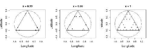
The as values span from 0.01 – 100, but the examples of as in figs 4 and 6 are really limited showing only 0.09 – 0.33 (ranks 7-12 out of 28 total). This also doesn’t include the grid mesh size which is the ‘switching point’ of behaviour (which I believe should be 0.38). When I have created the figures with a wider range of values it produces some interesting patterns not apparent from the current figures, and also makes much more sense of figure 8.

The ‘Spanning path length’ analysis –

This addition seems to be a bit of an afterthought – it is not described at all in the methods section and comes out of the blue in the results, with no indication as to the purpose of the analysis. Introduce the rationale for it and the methodology in the methods section, as it is important for the interpretation of the final figure.

Missing info in the methods –

As well as the distance analysis missing from the methods, there seems to be other key info not outlined in the methods and only apparent when going though the code. For example it is not clear from the methods whether there were any repeats, how many etc, and how they were averaged (working through the code I can see it is 30 reps but this info should be clearly stated in the methods). Please check that everything needed to replicate the study is outlined in the methods without referral to the markdown doc.

Fig. 8 legend –

All a bit messy. 1) What is the grid mesh size? What does centred mean if we don’t know what the extremes are? You may as well give the actual values (0.038 – 3.8, centre = 0.38 I think?).

2) Remove all the abbreviations (I’m not sure what ‘resp.’ means).

Fig. 4 and 6, maybe also other figures –

As well as indicating the most disordered value with a triangle, for the hybrid models you might consider having two symbols – one for the regular grid and one for random. Most people will really be only interested in the regular grid vs fractals, and so it is really worthwhile in every figure making it obvious where that regular grid lies. More minor, tweak the plot titles so that a[s] is in subscript

Figure 10 –

I’m not sure about the representation of the sampling area-budget arrows on the left and how easy it is to interpret. I see it is as more of a sampling area:no. sampling points ratio (more useful than sampling ‘budget’ I think, which depends on lots of other things). This then determines the FGM, which ultimately interacts with as. Perhaps that ratio can be defined by L as you have in the results, or maybe it is not generalisable in that fashion? Also, you could think about breaking it down for whether you are interested in estimating the autocorrelation mean or the range (or both).

Other trivial things:

Lines 333-337 – you could always use different coloured boxes to help indicate these

Sampling design figs 1, 2, 3 – v minor niggle but set asp=1 to keep aspect ratio of coordinates even

Line 50 – estimated ranges of what exactly, the autocorrelation range or distributional range?

Line 189 – ‘… accurately estimate …’

Line 220 – accurately what?

Line 445 - ‘… autocorrelation range was smaller …’

One final important point. I’m not Rob Ewers (I don’t have the beard for one), so make sure to remove his name from the acknowledgements.

Evaluation round #1

DOI or URL of the preprint: https://doi.org/10.1101/2022.07.29.501974

Version of the preprint: 2

Author's Reply, 09 Oct 2023

Download author's reply

Decision by Eric Goberville, posted 15 Jul 2023, validated 17 Jul 2023

Dear Dr. Laroche,

Thank you for submitting your article titled "Efficient sampling designs to assess biodiversity spatial autocorrelation: should we go fractal?" to PCIEcology. We have now received feedback from two referees, and I would like to express my gratitude to both referees for their thorough and insightful review of your manuscript. I share their opinion regarding the relevance of your study and its significant contribution to the existing literature, as well as the importance of providing access to the code for ensuring reproducibility of the analyses. However, before your study can be considered for publication, some revisions and clarifications are necessary.

The first referee noted that your article addresses a pertinent subject but highlighted a lack of references to recent research in the field. It is strongly recommended to include credible sources to support your arguments and enhance the credibility of your article. Additionally, the referee encourages you to delve deeper into specific aspects of your analysis by providing concrete examples or case studies to substantiate your viewpoints.

The second referee acknowledges the commendable aspects of the article, including the methodology of defining hybrid and fractal patterns and the use of the Pareto front method to examine trade-offs. Overall, the referee provides valuable feedback regarding the need to consider multiple variables/species, the practicality of sampling designs, and the choice of environmental variables. Further exploration of these aspects is encouraged to improve the practical applicability of the study.

We kindly request that you take these comments and suggestions into consideration during the revision of your article. Please submit a revised version of your manuscript, incorporating the referees' remarks. Additionally, we would appreciate a detailed response letter addressing how you have addressed the referees' comments.

Thank you for your valuable contribution to our scientific journal, and we look forward to receiving your response.

Best regards,
Eric Goberville

Reviewed by Nigel Yoccoz, 27 Jun 2023

Despite the recognized importance of sampling design, at least for researchers with an interest in statistical questions, it is remarkable that so few empirical studies in ecology are in fact designed according to well-defined objectives and some forms of random or systematic sampling. If one takes the example of species distributions, most studies use “available” data which are most often derived from opportunistic sampling or some form of hybrid designs (e.g. random design initially but with some nonrandom selection of final units linked for example to accessibility or observer availability). Many approaches have then been developed to account for this lack of design, but their robustness is often unclear. Clearly it would be preferable to start with a good sampling design.

This paper investigates different designs – random, grid, fractal (multiple scales) – and their efficiency when autocorrelation can be seen either as a “nuisance” and a parameter of interest. It is based on extensive simulations, and using a model-based approach for estimation. The conclusions are that fractal designs are seldom efficient. The scripts for running the simulations are available, but I did not run the simulations to check the results.

This is an interesting contribution for researchers working on sampling design, as it explicitly addresses different objectives (i.e. not “just” estimating population size, or an environmental effect). I could add that a specific difficulty with autocorrelation from a statistical point of view is that it may be hard to distinguish between a “real” autocorrelation due for example to intrinsic processes such as dispersal and the effect of a spatial covariate having an autocorrelation with the same range (i.e. it is not just an issue of bias but also of identifiability). As one often does not know what are the effects and range of environmental covariates, it is not obvious how sampling should be done. This paper addresses some of the issues associated with autocorrelation and estimating effects of covariates, and perhaps the author should emphasize the importance of making simulations to assess different designs depending on study objectives. Simulations are useful not just for assessing different design as is well done in this paper, but also because it forces the researchers to specify objectives, both in terms of ecological questions and in terms if what can be realistically expected in terms of precision/bias.