# Third review for "Predicting species distributions in the open oceans with convolutional neural networks"

I thank the authors very much for pushing further on this manuscript. I now find it clearer and more explicit regarding its findings (and limitations) and I am confident that will also be the case for other readers, making this hard work relevant.

Of course, this is all within the limits of not being able to re-run the analysis, but we all know that this becomes difficult once key people, students in particular, have left a lab. The ideas and general approach of the paper, by themselves, warrant its recommendation. 

I hope that the authors will continue this line of research and I am looking forward to reading further papers from them (although they may not be so keen in me reviewing them given the extensive nature of may remarks on this one and the time it took me to write them! Thank you again for bearing with me and I hope it will turn out to have been useful).

# Second review for "Predicting species distributions in the open oceans with convolutional neural networks"

## General remarks

My main remarks in the first round of review were:

1. the need for a baseline model to compare the CNN with
2. a discussion regarding the goal of this model and whether it was a "niche" model
3. the sometimes surprising choice of species
4. the fact that the model was a classifier, not a regression and that it could have unexpected consequences
5. the inclusion of geographical predictors (hemisphere etc.) which led to artefacts in the predicted distributions
6. the caricatural aspect of the 2ºC increase simulation

I understand that the authors are not in a position to re-run the analyses presented in the paper. This makes it impossible to fully answer some of my remarks or those of other reviewers. They made a significant effort to review what they could and modify the text. I leave it to the recommender to decide whether this is enough to warrant a recommendation in the end.

Regarding my main remarks:

1.
The addition of the punctual DNN is welcome and clearly shows the advantage of using the spatial information. This is a good addition to the paper. Thank you.

2.
This is now better presented in the introduction and the word "niche" is not used anymore in the context of this paper, which is appropriate.
The discussion of the fit with theoretical distributions (in section 3.2) is now more cautious.

3.
The selection of species could not be changed. The introduction was altered to mention that the species selected were expected to have different distribution characteristics.
Most are mobile species, for which the dynamic SDM approach makes sense. I still think including the Acropora coral, the only sessile species in the list, does not make sense, in particular in light of the following remark. 

4.
The nature of the model (i.e. a classifier) is now better presented, in a paragraph starting at line 206. A short paragraph in the discussion (line 345 and following) helps with the interpretation, but I think it is not enough, because the maps are actually very different from usual SDMs.

What is represented by each map is the *proportion* of each species among the 38 selected (assuming no sampling bias etc. as the authors point out).
This means the following, assuming a model with two species, A and B:
- in a pixel in which the conditions are maximally favourable for species A but absolutely not for species B, the value predicted for species A will be 1
- in a pixel in which the conditions are barely correct for A but still not favourable for B, the prediction will still be 1
- in a pixel in which the conditions are equally favourable for both, the predicted value will be 0.5 (as stated line 220)

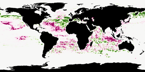
This makes it very difficult to interpret a single map in isolation from others. It also explains some of the very spotty aspect of the maps: when conditions are still favourable for species A but also become  favourable for another species, the predicted value for A drops. This is exemplified by the attached image [see PDF] where blue is for Caretta caretta, green is Carcharhinus falciformis and red is Carcharinus albimarginatus; while the whole region may be favourable for the green turtle, the extra favourability of some pixels for the sharks make the habitat suitability for the turtle drop. This is purely a numerical artefact, not an ecological feature: these sharks only rarely eat green turtles. This is not wrong per se, but it will likely be wrongly interpreted by an unprepared reader (I know I was mistaken during my first review and I only realised this now because we have been working with proportions too and scratching our heads trying to interpret the maps).

So, overall, it should be made much more obvious that all maps are maps of proportions among the 38 species (more frequently and strongly than the mention at line 246) and their discussion should be made in light of that fact. For example, the absence of a species within its distribution range (section 3.3) may be caused by differences in season, immediate vs. long term conditions, etc. as discussed, but also by the fact that another species dominates in one part of the range of the target species. Do not hesitate the repeat yourselves; it is quite difficult to wrap one's head around the interpretation of maps of proportions.

Another way to present this is to say that your model is not a model of species distribution but rather a model of *community composition*: you are trying to define the proportion of each target species in each pixel and, in particular, which one dominates. In terms of representation, to make this obvious, with few species, you could plot a single map with a colour in each pixel, resulting from a mix of colours proportional to the probability of each species; with three species, you could take Red, Green and Blue and the resulting RGB colour would inform on which species dominates. With 38 species, I am not sure what to do, but maybe you can restrict yourselves to a few?

In light of this fact, the selection of Acropora makes even less sense: all others share similar habitats, some may compete for the same food source, etc. It makes more or less sense to consider them as a community and study their relative abundance; this is not the case for Acropora.
It could have had little effect on the results since it is a very coastal species while the others are all pelagic (therefore their distributions are not "competing"), but that supposes that the coastal conditions are different enough from the pelagic ones, which is not true given its distribution map (and your discussion at line 415). This is briefly discussed in the new version of the paper but is a serious limitation for the predictions in the inter-tropical Pacific.

As you note, a way to circumvent this "relative abundance" problem is to predict many species at once: this was, each species is coexisting with, probably, many others in each pixel (i.e. each set of conditions), the predicted values do not approach 1 but their value is closer to the true habitat of the species. But the example above shows that 38 is not enough here.

5.
This is not presented as a limitation of the study. I am not convinced by the solution ("blurring" the limits rather than having hard ones): there will still be a fake boundary, which makes no sense to animals around the equator for example.
I was looking for papers discussing the inclusion of such specific geographic predictors in SDMs but could not find a definitive paper. This search probably needs to be deepened and the discussion of the consequence a bit more advanced (in the absence of the possibility to re-run the model).

6.
The simulation was removed, which I think was the right decision.

## Detailed remarks

56: While simple averaging indeed erases dynamic structures, it is still possible to use another summary in climatologies. For example, to predict the most favourable habitat of tuna, a climatology of the frequency of presence of fronts (from FSLE snapshots) is likely to be a relevant information. So add "If one uses simple averaging, the use of climatological..." and possibly rephrase this sentence a bit.

88: CNNs can be used for regression also, there is nothing specific to classification. I understand you added this sentence to highlight that *yours* is a classifier, but the current sentence is not specific enough.

133: Cleaning up species records was advised by another reviewer; you explained that it was impossible to perform all manually. I agree but some automated solutions could at least allow you to automatically spot outliers in geographical/environmental space (e.g. kernel density estimation).
Seeing some of the initial point distributions, this would be worthwhile, with Acropora records in Southampton for example...

Discussion: while I appreciate the effort to include many remarks from the reviewers in the discussion, they often only amount to an acknowledgement of a problem and a statement that this needs to be further explored. I would have preferred a bit more depth, in discussion in general

PS: draftable.com was super useful. Thank you for using it!

Predicting species distributions in the open ocean with convolutional neural networks.
version 2

# General comment on the revised version

During a first round of peer reviewing, and in addition to my review, the authors have received very thorough and high-quality reviews from the editor and from two other colleagues on the first version of the manuscript.

In this revised version, the authors did not rerun their model, nor changed their methodology, as this would have taken a lot of time, which several of them do not have because they are under short term contracts. While I totally understand this practical reason, I find that their answers to the reviews that they have received (in particular the very complete and constructive review of JO Irisson) are not as much detailed as the reviews themself. That being said, and if we accept the fact that rerunning the model is not possible for the present study, the authors have, in this revised version or their manuscript, addressed the comments they have received by modifying the text of the manuscript. They also have added, as a point of comparison to assess the performance of their model, new results from a non-convolutional neural network model as in Deneu et al (2021).

As a consequence, in this revised version, the manuscript is much clearer (e.g. regarding the classification task and species co-occurrences, regarding environmental variables) and the discussions is much more relevant scientifically and interesting for the readers. For instance, the Discussion section on "Suggestions to further improve the modelling methods" should be particularly inspiring for the readers.

Hence, since most of the comments raised previously have been properly addressed, I recommend this preprint after minor revisions.

See details below.

# Evaluation on how the authors addressed my comments in particular

Here I list the main concerns I had in the previous version of the manuscript and my evaluation on how the authors have addressed them in this revised version:

1) Main concerns on the description of species occurrences and environmental variables in the Method section => The Method section is much clearer now. I still have one comment: the authors state in their response that "We provide the source for each variable in table 2, which includes their unit and many more information", while the units are still missing. Please add them in table 2.

2) Problems identified in the predictions: the way co-occurrences are handled is clearer now and the way the results are presented and discussed has also been improved.

3) Limited relevance of the "SST+2°C" scenario: This problematic part has been removed in the revised version.

4) Choices of 38 taxa: I totally understand that the authors do not which to re-run their models and I am fine with their answers.

5) Relatively superficial discussion: the scientific relevance of the discussion section has been significantly improved.

6) The conclusion section also lacks strong scientific background: the conclusion has also been improved and is now satisfactory.

7) Minor comments: they have been addressed, except the following that was not understood: "Line 105: essential to?" => line 123, replace "which is essential to reproducibility." by "which is essential for reproducibility."

# Miscellaneous comments

## Minor comments

As usually done, the authors could acknowledge the reviewers and editor/recommender for their help in improving the scientific quality of the manuscript. Such acknowledgments would seem especially fair in particular given the thorough inputs provided by Jean-Olivier Irisson.

- line 171: "Because we propose a type of dynamic SDM, we cannot capture these long-term barriers, so we have to include them artificially." Alternatively, could you have considered using longitude and latitude? Or do you think it would have been a problem due to observation bias (as mentioned line 179)?

- Comparison between the CNN and punctual DNN: could you provide a rough estimate of the computing cost of each method? Is the confusion matrix similar? Are they some species that are better captured by the CNN, or is it due to a better performance of the CNN for all the species? Looking at Table 3, one could also argue that the increase in performance when using a CNN compared to a punctual DNN is not so high.

## Suggestions for text editing:

- line 89: I suggest removing "as is usually the case with SDMs"
- lines 96-97: Replace "Here we present an adaptation of their work that includes these adaptations to the specificity of the open ocean." by "Here we present an adaptation of the work of Botella et al. [22] and Deneu et al. [23] that includes these adaptations to the specificity of the open ocean."
- line 152:  Add a reference to Table in 2 the sentence "the oceanographic landscape that we consider has limited precision due to environmental data resolution".
- line 139: "Three of them contain two components: surface wind, geostrophic current and finite-size Lyapunov exponents (FSLEs)": do you mean zonal and meridional components? It seems later on (line 314) that it is rather polar coordinates ("strength" and "orientation"), but then in Tables 2 and 4 it is indicated that cartesian coordinates (u,v) have also been used. Please be more explicit line 139: "Three of them contain two values: both strength and orientation components (e.g., polar coordinates) for finite-size Lyapunov exponents (FSLEs), and both zonal and meridional components for surface wind and geostrophic current".
- line 156: "115km" => "115 km"
- line 164: "7km" => "7 km"
- line 239: "100 km" => "100 km" 
- Figure 4 and Figure 8: If possible, the species names should be in italic.
- Caption of Figure 5: "chosen because they deserve commenting" => "chosen to further discuss some interesting and contrasted patterns".
- Figure 8: would it be possible to order the variables according to their order in Figure 7?
- line 358: "A way to improve the final accuracy score would be to group species by traits": I am not so sure that species with similar traits are more truly observed more frequently together, since species also coexist in functionally diverse communities. Consider rephrasing, for instance "to group species by habitat preferences"?
- line 403: "As previously discussed, this method would probably benefit from including a large number of taxa. In particular, planktonic species may prove valuable as they are less prone to sampling biases" => I would also argue that they are several databases of plankton species occurrence available for SDMs, as the ones developed at ETHZ, such as the 1704 species compiled by Righetti et al. (2020) or the 524 zooplankton and 336 phytoplankton species compiled by Benedetti et al. (2021) for SDMs:

D. Righetti, M. Vogt , N. E. Zimmermann, N. Gruber, 'PhytoBase: A global synthesis of open ocean phytoplankton occurrences', Earth System Science Data, 12, 907–933, https://doi.org/10.5194/essd-12-907-2020, 2020

Benedetti, F., Vogt, M., Elizondo, U.H. et al. Major restructuring of marine plankton assemblages under global warming. Nat Commun 12, 5226 (2021). https://doi.org/10.1038/s41467-021-25385-x

- line 430: Regarding the "spotted aspect of the map", I wonder if another pixel size for oceanic environmental variables could be more adapted for the 32 × 32 geographical pixels, compared to what has been done here inspired from terrestrial environments, e.g. for specifically targeting submesoscale features. Cf. for instance Lévy et al. (2018).

Lévy, M., Franks, P.J.S. & Smith, K.S. The role of submesoscale currents in structuring marine ecosystems. Nat Commun 9, 4758 (2018). https://doi.org/10.1038/s41467-018-07059-3

Thank you to the authors for a very thorough response to my review and those of the other two reviewers. I felt that the discussion on both sides of the review was very helpful and has significantly improved the revised version of the manuscript. I have reviewed the responses to each of the reviews and the revised manuscript and am overall happy to recommend it be advanced (with minor/line edits) to acceptance from my perspective.

My largest issue (which was echoed by Reviewer 1) was related to the formulation of the prediction problem as a multi-class classification problem. I appreciate the authors’ response to this point in their responses to both reviews and the addition of the new text highlighting this difference between their approach and a more traditional approach. I understand the authors’ argument that this perhaps generalizes to predicting the relative detection rates of each species though I think the assumptions needed to get there are unrealistic in the general case. Regardless, I still believe this family of frameworks are on the rise and am happy to see this paper contribute to the general discussion of the technique as a whole, given that the authors have added a good amount of clarity around their methodology here.

Reviewer 1 makes several arguments about the focus/scope of the method and discussion, which I agree with and think the authors have done a satisfactory job resolving. I believe the revised draft of the manuscript is more concise and clear as a result and at no significant cost to its potential impact.

Reviewer 1 also makes numerous suggestions which could improve the analyses and which the authors have generally decided to incorporate into the discussion to setup future research lines for follow on work. I am of the opinion that in general these potential improvements are appropriate for future work and generally should not preclude the publication of this work and appreciate the authors’ effort to transcribe these suggestions into the manuscript.

Given that the authors have indicated their aversion to significant revisions to their methods or results, I’d like to say that I am personally satisfied with the experiments that they’ve performed and am not overly concerned that their resulting discussion is misleading or that a reader might be misled about the approach as a result of the experimental setup the authors’ have presented.

Line items
L91: optic → optical

L93: Chlorophyll → chlorophyll

L144: rephrase → “were encoded as layers with equal dimensions to the other variables.”

L190: typo: explicitely

L273: cut

Fig5 caption: cut “chosen because they deserve commenting.”

L329: coherent → consistent

L351-355: I’d cut this attempt to justify any poor accuracy of a dynamic model via movement or individual stochasticity

L426: “one if the” → “one is the”

Once again, thank you to the authors', reviewers 1 and 2, and the editors for the interesting paper and discussion. I again appreciate the opportunity to review this very nicely written manuscript.

# Review for "Predicting species distributions in the open oceans with 3 convolutional neural networks"

This article uses the method defined by Botella et al (2018) and Deneu et al (2021) to model the occurrences of 38 marine taxa based on a new set of environmental variables appropriate for this environment. This is a very good idea since this method seems extremely promising and should be relevant to capture important mesoscale features in the ocean, such as fronts.

Furthermore, the authors should be commended for the effort they made to make their research reproducible and reusable by others. They shared the input data, the results but also the code used to fit the model and the code to extract relevant environmental data around a point of interest, in the form of a Python package. This is excellent.

While I find the premises of the study interesting and its technical setup exemplary, I have several remarks about the content, which I detail below. I hope that they will be perceived as useful by the authors.

## Major remarks

### Baseline model

In quite a few ways, this model is different from that of Deneu et al (2021): the species and environment are different of course, but also the way the missing values are handled, possibly the loss function, the evaluation metrics etc. For all these reasons, it would be necessary to evaluate the results against a baseline model. It would help highlight the advantage of using a CNN and substantiate such claims in the discussion: "This method holds promise in helping researchers uncover new correlations between the oceanic conditions and species distributions".

The comparison that would best show the potential advantage of adding the convolutional part would be with the "Punctual deep neural network (DNN-SDM)" of Deneu et al, keeping the dense part exactly identical to the one used in the current model.

An alternative that would allow comparing with a "classic" approach would be to predict each species independently with Gradient Boosted Trees (or a Random Forest) and pseudo absences at the points of other species.

Yet another alternative that would keep the multivariate response but use classic tools would be to use Gradient Boosted Trees in a classification setting, with categorical cross entropy loss (`logloss` for xgboost).

### Is this model a Species Distribution Model?

55-56: "Furthermore, SDMs rarely take into account the high temporal variability of environmental data [14], which seriously hinders the prediction of highly mobile species distributions."
This, and other aspects of the paper pose the question "what is a niche" and whether the model trained here is a niche model. The ecological niche of a species is the set of conditions in which this species can survive and reproduce; it is shaped by natural selection. The purpose of a Species Distribution Model, or a Niche Model, is to capture that niche and project it spatially, as the region in which the species should be found, i.e. the distribution *range* of the species. A reason why most SDMs use climatological summaries of the conditions in a given place (mean, but also min and max, etc.) is because the presence of a species in a given place on Earth is not determined by the immediate conditions in this place but by the long-term range of conditions experienced there. This is easily understandable for non-mobile species: the persistence of an oak forest depends on the range of conditions experienced over the last decades, not on the temperature at any specific date. Even for mobile species, the purpose of a SDM would still be to project the complete range of existence of that species; its extent would be determined by natural selection, again, not by the individual movement ability of the organisms.

I would argue that a model that relates the presence of organisms to the immediate, dynamic environmental conditions of a given place, as done here, is not a "niche" model anymore. A broader term in which this could fit would be "habitat models". It uses the same general reasoning (organisms are constrained by their environment) and often the same statistical tooling, but the underlying hypothesis is different: while in niche models, the presence of a species in given conditions is to be related to its ability to persist in those conditions over generation, here, the presence is determined by the organisms ability to move towards favourable conditions at a specific time of the year (or rapidly multiply in these conditions, but all animals here are long-lived so this does not apply). In passing, this makes the non-negligible hypothesis that the animals in question have the ability to detect those regions of favourable conditions from far away (through direct mechanisms or proxies) or at least to sense when they are in bad conditions and move away from them.

I would like to this this question discussed in the paper and, while you can refer to niche models as inspiration and regarding their general principle, I think that the mechanisms represented here do not pertain to the ecological niche of the species and this should be made explicit.

This would have implications for section 3.2, where you compare a snapshot distribution over one date (March 2021) to the map of the distribution range of the species. It is unsurprising that they do not match and you cannot even hypothesise from them that "the established geographical range is not fully used by the species". I suggest that you can:
(1) either use those maps to check that the distribution you predict is *within* the range of the species, as a broad check of the method, and not more;
(2) or predict those maps for several seasons of several years (probably 20 to capture a full climatic period), produce an average, and then compare this average with pre-existing species distribution maps.
I assume solution 2 is computationally very demanding.

The discussion should also be reviewed in that light. Part 4.1 compares this to SDM studies and conclusions such as "This highlights the need for distribution models of fast-moving species to consider these variations, instead of relying only on averaged values" are misleading. It is just that habitat models using snapshot of dynamic fields vs. average fields do not answer the same ecological question at all. If one wants to model the distributional range of a species, then climatological averages *are* the correct answer (or possibly averages of snapshot predictions over climatological scales).

### Choice of species

Related to the points above regarding the nature (SDM or not) of the model, I find the inclusion of the Acropora coral very strange in this list. All other species are large, quickly moving organisms, which could indeed follow water masses of suitable properties; therefore what is modelled is the set of favourable conditions throughout the year (rather than the niche). This relates to "movement ecology" to which you refer a couple of time. In the case of Acropora, the relationship between presence and immediate conditions in the vicinity (in time and space) of the observation make much less sense; for this taxon, the long term conditions are what determines species presence. While your model may still capture the fact that Acropora lives in rather warm waters, for example (because no occurrences will be recorded beyond tropical regions), a model based on climatologies would make much more sense. I would suggest to remove it. I realise that it means re-running all model fitting and predictions, since the model fits all species together...

Furthermore, it would be relevant to justify the choice of species in the text. Again you seem to have made a deliberate choice of large, wide ranging/moving species, state it, explain why, and draw the conclusions for what your model is about (see above).

### The model is a classifier

While the model is presented as predicting species distribution, which is usually seen as a regression problem, it is actually a *classifier* that predicts which species, among those modelled, is the most likely to occur in any given pixel of the ocean; and there can only be one. As the authors briefly discuss (286-290), this is problematic when two species occupy the same environmental space and should therefore be equally likely to occur in a given pixel. The probelm appears for the accuracy metric (which is what the authors discuss in section 4.2.1) but is also, and more profoundly, affecting the model itself.

If two species occur in the *exact* same conditions (i.e. in the exact same places and times, in the context of this paper), then the model has no way of sorting out these contradictory informations and will come to a 50-50% answer, which is the right one.
Now, in the more realistic case where two species occur in very similar but not exactly the same conditions (for example, close to each other geographically), they should still be predicted 50-50%. However, the softmax and cross-entropy loss will instead push the model towards extreme answers in terms of "probability": to minimise the loss, not only should the model predict the correct one of those species in a given pixel/set of conditions, it should also predict it with high probability, and therefore all others will have low probabilities. To achieve this, the model will pick up minute differences in conditions, that are probably irrelevant biologically, and output predictions that are far from 50-50%. I would venture that this is one reason for the very spotty aspect of the predicted maps, in the Indian ocean for _C caretta_ or the west Pacific for _P pacificus_ for example (one other reason may be mesoscale structures that would be visible in the FSLE, temperature, etc. but it is difficult to say without a map of those). Actually, this could even be the reason why FSLE is one of the most predictive variables: it has very strong local structure and therefore is one variable that can be exploited by the network to come up with (artificial) differences between nearby occurrences.

Unfortunately, I do not have an easy solution for this. Deneu et al, who use the same approach, get (probably partially) around this problem by predicting a very large number of species (>4000), which likely helps smooth things out during training (especially is sufficient regularisation is used), and use metrics that consider the top k predictions only (not top 1), which diminishes this issue during evaluation. This is not applicable for you. Maybe another loss function would be more appropriate in your case?

A common solution to reconcile disagreeing inputs in SDMs (e.g. presence and absence of the same species in similar conditions) is binning. Because the models operates in environmental space, such binning should ideally be done in the n-dimensional environmental space. However, it is commonly performed in the 2-d geographical space because it is easier and has the added benefit of correcting some of the observation bias (reduce the number of inputs in regions frequently observed; as noted in your section 4.2.2). In your case, the environmental space is only defined after the inputs pass in the feature extractor and it has likely >1000 dimensions (the output size of Resnet50); so using this is out of the question. You consider geography *and* time to fetch the environmental data, so binning should be 3-d (lat,lon,time), not 2-d as usual. The idea is then that, if you get observations for two species relatively close in lat,lon,time then you consider them as a single input with two 1s on this row, hence capturing the fact that these two species co-occur. For this to happen, your bins probably need to be quite large and one possibility is to consider only the week or month of the year for time. This should also be done on the full GBIF output, before the subsampling of 10,000 per species. From then on, the loss function should cope with the fact that there can be several 1s on the same input; I do not know enough about cross entropy to know if it does. MultiR2 would but has other drawbacks. 

Overall, (i) the fact that this model is a classifier and the meaning of predictions should be made clearer in the text, right from the abstract and introduction, (ii) the effect that this fact has on the predicted maps should be discussed more, unless, of course, (iii) an alternative solution is found (through a different encoding or loss function).

156-171: as a side note, you mention using binary cross entropy although your response has length 38, not 2; you are probably using categorical cross entropy, like Deneu et al, right?

### Geographical predictors

136-140: I am ambivalent regarding the inclusion of the geographical variables justified by the fact that they constitute barriers. If this is considered a SDM, the barriers should have been present for a sufficient amount of time in the evolution of the species to let subpopulations evolve different preferences in the different basins and this is not mentioned/justified. If it is not a SDM but a "preferred habitat" model (which I think it is), the reader is still lacking justifications that most species do not regularly cross these barriers. But most species considered (tunas, marlins, sharks, whales, dolphins, etc.) have global distributions and, while they are often managed/considered as different stocks, they likely could move from one ocean basin to the next. For the model, the question becomes whether these subpopulations have different environmental preferrenda in those various basins, warranting the inclusion of those variables to capture interactions with other variables (e.g. different temperature range in the Atlantic vs Pacific). I do not know enough about the biology of all species to be conclusive but I think the authors need to justify that choice further.

The most problematic choice is the inclusion of hemisphere, which creates a completely artificial boundary in the distribution of _Caretta caretta_ in the Indian Ocean (Fig 5a) for example. I understand that was included to avoid predicting arctic species in the antarctic but the artefact above is reason enough to remove it, in my opinion. Maybe the arctic/antarctic separation can be ensured by masking on the prediction: setting the proba of arctic species to 0 for all points in the southern hemisphere, or south of a given latitude, and rescaling the others to sum to 1?
Sidenote (related to line 144): the polar front is a pretty strong barrier for many species, even though it is not "physical" in the sense of a continent. If the warm waters of the equator are considered barrier to movement, then this could be also, which makes including hemisphere even more questionable.

Finally, if I understand correctly, these binary variables were included by giving a completely uniform 32×32 input tensor (filled with either 1 or 0, I suppose). First, this wastes a bit of computational resources since performing convolutions/pooling on a constant input just outputs the same number. Second, I am not completely sure how those would behave during the convolutions with the other tensors (i.e. other variables) but it is likely that tensors of 1s just have no effect while tensors of 0s mask the other variables. In both cases I think this is not what you want: you want the effect of the patterns in the other tensors to be *conditional* to the geographical variable, e.g. you want the temperature patterns to always show but have a potentially different effect in the Pacific vs. Atlantic ocean. Furthermore, in the first layers of the network, the convolutions of those constant tensors will be limited with the tensors that happen to be placed next to them in the 32×32×29 stack, which, again, is probably not what you intended.
For all these reasons I suggest that, if some geographical info is to be kept, it should be included as additional scalar values (of 0 and 1) concatenated to the output of the feature extractor, i.e. in the first layer of the Multi Layer Perceptron. This way, they are not used in the convolutions and they can interact with all other variables through the fully connected layers.

### 2ºC increase simulation

I do not find this section useful. You acknowledge yourselves that more than temperature will change in the future. So just adding 2ºC everywhere, without considering the associated change in stratification, circulation, primary production, etc. is just unrealistic.

The minimal relevant way to do this would be to consider full earth system models outputs, for at least one model and one scenario, to fit and project the model in the present and project it on the future time (both taken from the same run!) and compute the difference between present and future. More appropriate studies would transform the climate model to fit in the space of observations, using something like CDF-t, and to fit+predict the occurrences in this new space, in both the present and future, for different earth system models and scenarii. This is clearly out of the scope of this study. So this part should just be cut.

## Minor remarks

Abstract: "for prospective modelling of the impacts of future ocean conditions on oceanic species" : nowhere in the Abstract is the +2ºC experiment mentioned so the reader cannot know what this sentence refers to. But see above regarding the relevance of this +2ºC experiment.

15: Ref [1] applies to the deep ocean, not to the surface; it is not be the most appropriate to justify this sentence.

25: the influence of temporal variations: what does it mean exactly? At this point the reader has not read about the time resolution of the study and similar models frequently use climatologies, hence erasing time. It would be necessary to explain a bit more.

26: identify areas that are most at risk: risk of what? SDMs can predict species distribution but then, from that, how to identify regions at risk or not? Rephrase.

79: (about Sentinel2 data) "we cannot rely on this information in the open ocean": why? Sentinel-2 data is readily available and can be used to describe, in great detail, phytoplankton blooms for example. The product derived from Sentinel's raw data make most sense on land (to capture vegetation cover etc.) but the raw RGB data can be used at least.

94-95: at this point a few sentences should be added about the fact that the response is multivariate, otherwise the reader cannot understand why the output of the model is "a vector of observation probabilities". The most common approach in a species-environment model would have been to make one univariate model per species.

108: GBIF data being what is it (invaluable but sometimes worsened by records of lower quality), I am very surprised that you did not have to further clean the data. If you did inspect it then please mention what you did. If you did not, I think it should be checked for:
- duplicate records (including with a buffer around each point since the duplicate may have slightly different coordinates)
- records that are far out of the geographical distribution of the rest of the points and that are likely to be mis-identification or wrong geographical coordinates; this can be done with density-based methods.

131-134: the change in lon/lat ratio when moving from the equator to the poles is acknowledged but how was it taken into account? Was is considered when performing the interpolation from 241×241 to 32×32?

Table 2: some choices in environmental variables are strange.
Why take Chlorophyll from a source (33) different from that of the phytoplankton groups (35)? Chlorophyll is actually available from the same Copernicus product and using this would ensure a more consistent signal among the this and phytoplankton functional types. This would avoid having a signal for phytoplankton groups but missing data for Chl --which then appears replaced by the median-- as visible in Fig 3.
Why consider u,v for wind and current but strength and orientation for FSLEs? I think the relevant choice is strength and orientation for all; this is what animals will more directly be sensitive to. Furthermore direction is an angle, meaning that, in its raw form, slight changes from 359º to 1º would appear as a major feature/ridge in the 32×32 tensor (as is visible in Fig 3 actually) and this artefact will be picked up by the convolution filters. It should be transformed to be continuous. Common transformation for angles are logit or cos and/or sin.

Regarding environmental data, what is the time resolution of the products? Was any time-wise interpolation done to define the array of values taken or it was just the closest available date? If it is the later, knowing the time resolution is particularly important.

150: what does "clipped" mean: replaced by a missing value (and therefore replaced further by the median) or replaced by the previous most extreme value?
153: you used the median to fill in missing values while Deneu et al (2021) mention "Furthermore, rasters contains sea pixels and other undefined values that should be attributed a numerical value. To avoid as much as possible potential errors related to this constraint, we chose a value sufficiently distinct from the other values, here we choose a value under the minimum of the values of valid pixels". And indeed, in your case, when pixels are land for example, they should probably get a different value which would allow the model to pick that up. Can you justify the choice of the median vs. the choice made by Deneu et al. above?

174: how was the 80-20-20 split done? Given the origin of data, there may be autocorrelation among the data points (several occurrences reported in close proximity in space and time). Not taking this into account by doing a purely random split would
(i) push towards overfitting (if points in the validation set are close to points in the training set, fitting tightly to those points in the training set would decrease validation loss) and
(ii) inflate accuracy (if some points in the test set are close to some in the training set, they are "easy" to predict).
Common solutions to this are block cross-validation, withholding of complete regions (in space-time for you) for val/test, or choosing points that are far from others by examining the density of observations and picking points in low density regions.

192: what are the resolutions of the prediction grids in both regions, in degrees? What resolution was it interpolated to afterwards? How (linear, spline, other)?

194: is there any clever trick in the fetching of environmental data on a grid? Indeed, it is likely that the regions around successive grid points overlap and therefore that it is possible to fetch a large region once and then cut it into chunks rather than downloading each one separately (leading to multiple downloads of the same pixels). If such cleverness is built into geoenrich, mention it, it is worthwhile!

197: can you make it a little more explicit what you mean by "relative probabilities"? Probabilities sum to 1 for each pixel, by definition, so what does the added "relative" mean? My understanding is that, in the maps, the probabilities of occurrence are rescaled per species, so that, even if a species has a low probability of being the first predicted species everywhere, the map still goes from white to dark blue. Is that the case? If so I would call them "rescaled probabilities"; or I would just display the probability but keep the colour scale independent for each plot (no matter if the max is 0.9 or 0.01, it is dark blue).

208: the general principle of the "integrated gradients method" would need to be explained here. It is not well known enough to assume that readers will know what it does and it would be nice to avoid them having to read the underlying paper to understand it.

209: how representative is this 1000 random sample? Was it stratified geographically to ensure it covered various conditions?
Ideally, these 1000 points should cover enough of the environmental space of the full 36506 to be considered representative. One way to check this is to extract the feature vectors of the 36506 points (i.e. the values at the end of the feature extractor, or possibly at a further layer of the MLP), draw the density distribution of values for each feature, do the same with only the 1000 and compare the density distributions. You want those to match as best as possible. The mismatch can be quantified with the Kolmogorov-Smirnov statistic, for example, and deciding whether 1000 is enough can be done by using 10 (which will not be enough), then 100, then 500, etc. and check when the statistic saturates.
A cheaper and approximate way to do it is to extract only the centre pixel for each variable and do the same: i.e. does the distribution of temperature at the 1000 points look like the worldwide distribution.

210-211: I am not sure I understand this. The summing over geographical area would tell you if the most explanatory variables are similar between the Atlantic and Pacific for example, right? But those results are never shown. Then the sentence suggests that it is the values aggregated by area that are then summed per taxon, but Fig 8 is only per taxon; I assumed this was just a straight sum over the 1000 points.

Section 3.2: on several occasions, in that section, you explain the geographical discrepancies between the theoretical distribution and the predicted one by under-representation of occurrences where the species is not predicted (l. 232, 241). But the model operates in environmental space (except for the few geographical variables) so the representation that matters is that of the environmental conditions, not of the geographical locations. This is actually the whole point of such habitat-based models: predict probability of occurrence in data poor region. So you should be a bit more careful with the wording here (in addition to reconsidering the general point of view of this section, as explained above).
NB: This is also one more reason to avoid adding geographically constraining variables.

280: the fact that the effect of variables has to be studies afterwards is not a drawback of solely this method. It is the case for all other machine-learning based methods (where partial dependence plots have to be drawn after model fitting) and even multivariate linear models where the true understanding of the contribution of variables come from effects plots. It may be longer and more computationally demanding to undertake here, because of the complexity of the input data, but is not different conceptually.

302: "The strength of deep learning in this context is that it makes no assumption when there is no data: it replicates the results from similar well-known areas.  This partly compensates for sampling effort heterogeneity." This is true for habitat models in general (it is actually the purpose of these models); there is nothing specific about deep learning here.

304: "But this only works when there is a homogeneous population". Actually, this model (and other machine learning-based ones) likely has enough degrees of freedom to capture multimodal responses. So if a species has two stocks, which respond differently to environmental conditions, the same model should still be able to capture both relationships and predict presence in all places that are favourable in at least one of the two stocks. But of course, one needs samples from each stocks to start with. For _T thynnus_, the issue is likely the imbalance between the West and East (only ~900 occurrences east of -35º, over a total of ~9000). So, overall, this is a data problem, which fits in this "Observer bias" section, but the wording makes it sound like a model problem.

Section 4.2.3: pointing what the model missed is good and honest. But the reader is expecting explanations as to why this was missed. Is it a lack of occurrence data, the lack appropriate environmental variables relevant to capture the conditions towards which the animals migrate, a problem with the fit of the model?

Section 4.3.3: This is relevant and, indeed, an interesting perspective. But how would you deal with pixels on shore in that case? This is related to my enquiry above regarding the use of the median value to fill missing values, which differs from Deneu et al.

335: this sentence is actually true of all habitat models. You should make it a bit more specific.

## Specific corrections

Abstract: due to scarce observations -> due to the scarcity of observations

Abstract: observations, and -> observations and : in general, there should never be a comma before and in an enumeration of two items. Please review throughout.

Abstract: 38 taxa which include -> 38 taxa comprising : "which" should introduce a sub-sentence and be separated from the main sentence by a comma.

Abstract: mammals, as well as marine -> mammals, marine

Abstract: this black box model -> this purely correlative model : black box is a bit of a catch-all term. The model is not so black box after all, since you can get insight into which variable is most explanatory. I would avoid the term

Abstract: insight for species-specific movement ecology studies : why "movement" in particular? 

16: climate, nutrient cycles, and biogeochemical cycles : remove nutrient cycles, it is redundant with biogeochemical cycles.

22: To focus on solving -> To solve

22: it is essential to -> a necessary first step is to

23: the open oceans -> the open ocean. "Open ocean" is a general term here, not designating any single ocean in particular. Change everywhere.

37: There is a wide -> A wide variety of Species Distribution Models (SDMs) have been discussed

38: environmental niche: the area where : The niche is defined in environmental space; it does not designate a region, it designates a set of conditions in which the species thrives.

40: with specific environmental conditions : I don't understand what this part of the sentence means.

41: where the prediction is computed -> where the observation is recorded

43: area does not -> area would not 

44: seamounts or trenches. -> trenches for example.

46: these spatial structures are essential to understanding species distributions -> these spatial structures represent processes essential for determining species distributions

48: include the values of these environmental data -> include the environmental data

49: variables -> predictors

51: summarize input data as fewer significant variables -> summarize input data into fewer relevant variables

51: made manually -> carried out manually

60: invented -> designed

62: image classification -> image processing

66: objects is probably enough

71: at the point of occurrence -> at a given point : this is relevant also for prediction

72: temperature fronts -> fronts : there are salinity-driven fronts which are equally important

81: relies only on environmental data : isn't Sentinel-2 data environmental data? Rephrase.

83: we explore and report the possibilities -> we explore the possibilities (or we explore and report *on* the possibilities; but explore is probably enough)

91: to build a model to link environmental data to species presence. -> to build a model to relate species presence to environmental data.

92: we used freely available occurrence data -> we used occurrence data : the env data is also free and nothing special was mentioned about it.

Fig 1: Point grid -> Grid

102: large pelagics -> large pelagic fishes (or something else but pelagic is an adjective, it requires a noun).

103: delete "These taxa may be replaced or complemented with others in the future"; you say it in the conclusion and it has its place there. 

108: move "Furthermore, convolutional neural networks are known to be 109 robust against occasional labelling mistakes [19]." before "We removed..."

111: When there were more than 10,000 occurrences of a taxon, a random sample -> When more than 10,000 occurrences of a taxon were available, a random sample : overall, "there is" is to be avoided in written text; please check throughout.

126: and made available -> and is made available (and congrats again for packaging this and making it available!)

Table 2: please group similar variables together (e.g. SST, SST -5d, SST -15d). Please mention from which type of source Eddy kinetic energy is computed (I assume models).

Fig 3: like in the table, keep related variables together, to ease comparison.

178-180: those are results and should be placed there; possibly in the section about quality assessment of the model (3.2).

178: those statistics are on the test set? If so, state it explicitly.

182: easily identified -> well predicted

Fig 4: formatting numbers >0 with leading zeroes (001 instead of 1) is slightly misleading visually (the number of errors "looks" similar between 001 and 999)

Fig 6: what do you mean by "the contrast was increased"? Does it simply means the colour scale is not the same as in Fig 5? If so, use a different colour, it will make it more natural. Is it still the same for all panels of Fig 6?

Table 4: Redefine the quantity displayed in the legend of the table. Also, the values are sorted by median but the mean and standard deviation are also reported. If the distribution of values is such that the median makes more sense than the mean, then report only the quantiles (not the mean) and the median absolute deviation (instead of the standard deviation).

267: The variables that were identified are -> The variables that were identified as important are

268: important movement predictor -> important predictor of movement

269: I suggest adding the part in brackets: "Sea surface temperature was also expected to be an important predictor, [since it has important physiological consequences and is therefore] the most frequently used descriptor in." SST is not important because it is widely used; it is widely used because it is important. 

273: two final periods. Remove one.

286: what does "depending on the ecological context" mean?

322: I think what you mean here is sourcing from different datasets within GBIF instead of randomly. But this is not obvious and should be rephrased.
But, again, binning would be a better way than resampling and would correct some the sampling bias.

335: species distribution at all and all areas -> species presence at all dates and all areas

## Conclusion

Overall, while this work is a valuable contribution, has the potential to be a very interesting one, and could prove seminal for the future of such approaches, I cannot advise for recommending it at this point. At the very least some points need to be discussed more in depth and it is  likely that some computation needs to be added/redone.

I would be happy to interact with the authors if some of my remarks are not clear enough.

Thank you to the authors for an interesting and exciting article and to PCI for the opportunity to review it! Additionally, I'd like to thank the authors for the impressive commitment to making their code, data, and manuscript publicly available. My review is below.

### Summary of Article

The authors present a multi-species, temporally explicit SDM built using typical CNN methodologies for a broad suite of 38 marine species and genera using data from GBIF. The CNNs were built using 25 environmental variables at varying spatiotemporal resolutions and the output layer of the model was configured to output the predicted probabilities of each taxa, which were then interpreted as two primary forms of species distribution prediction. Finally, the authors conduct a variable importance analysis of the environmental variables using integrated gradients. They conclude with a discussion of potential future work and improvements for the model and their results.

### Summary of Review

The authors' article contributes to a hot topic exploring the application of deep learning to species distribution modeling. There is, I believe, a common philosophy that DL (and specifically CNNs) should be a clear winner for SDMs and a reasonable value proposition in understanding which domains are more or less suited to being modeled via CNNs and still little collective understanding of best practices when following this approach. I have some suggestions for critical details that should be described in the manuscript, and key questions about the interpretation of the results, but I support the fundamentals of what the authors have done here and believe it could be a particularly valuable contribution to the literature even if only my simpler feedback was addressed.

Overall, I'd recommend this article be revised and resubmitted.

### Major feedback and questions for the authors

* Did you use a pretrained resnet-50 model? If so, which?
* How was your model extended to a 29d input layer? This is not a trivial extension of the Deneu or Botella models and the new architecture should be described more completely.
* Additional detail is needed on the alignment process for environmental variables, particularly for variables that were downscaled. It should be clearer throughout the manuscript what resolution was being modeled.
* I have a fundamental issue with the treatment of model predictions as a multi-class classification problem, including the one-hot encoding of training data and the interpretation of the predicted class probabilities. In particular, the "accuracy" of predicting the most likely species within each pixel follows the GeoLifeCLEF problem formulation and is fundamentally problematic, particularly when modeling with presence-only data from GBIF. Additionally, treating the predicted class label probabilities as a surrogate for suitability or RPoO and presenting spatial visualizations of these probabilities as a snapshot SDM is a misinterpretation, in my opinion. This space is still being defined within the literature, so I wouldn't object to publishing this treatment, but I would encourage the authors to at least address this treatment of presence-only SDM data in their discussion of the interpretability of the distribution predictions.
* The authors dismiss the need for data cleaning because of the robustness of CNNs to mislabeled or erroneous records. However, recent studies (Zizka et al., 2020) have estimated the proportion of problematic GBIF records to be as high as 41-44% of all records. I'm not aware of a paper which has investigated the robustness of CNN-SDMs to GBIF errors and so would encourage the authors to reconsider this lack of data cleaning for their model.
* I like the description in §1.3 of how CNNs pool feature detectors at varying levels of coarseness and how that might be paralleled in a climate/environmental SDM. However I think the language of what is happening as the models learn different weights for the convolutional layers is imprecise and could mislead readers. It would also make an excellent conceptual figure, space and time permitting.

### Minor feedback and line items

- §2.7: Why were some variables removed apriori before variable importance?
- "Figure X", "Table X", and "Section X" should generally be capitalized throughout the manuscript (e.g. on lines 103, 111, and 115)
- The term "probabilities predictions" is used a few times throughout the MS (e.g. L87) and should be replaced with "predicted probabilities"
- L51, "This work may be made manually": doesn't scan for me, perhaps prefer "These summary variables may be constructed manually by experts, ..."

Again, thank you to the authors for the opportunity to review their impressive project and I look forward to seeing it in print soon!

References

Botella, C., Joly, A., Bonnet, P., Monestiez, P., and Munoz, F. (2018). Species distribution modeling based on the automated identification of citizen observations. Applications in Plant Sciences, 6(2), e1029. https://doi.org/10.1002/aps3.1029
Deneu, B., Servajean, M., Bonnet, P., Botella, C., Munoz, F., and Joly, A. (2021). Convolutional neural networks improve species distribution modelling by capturing the spatial structure of the environment. PLoS Computational Biology, 17(4), e1008856. https://doi.org/10.1371/journal.pcbi.1008856
Morand, G., Joly, A., Rouyer, T., Lorieul, T., and Barde, J. (2024) Predicting species distributions in the open ocean with convolutional neural networks. bioRxiv, ver.3 peer-reviewed and recommended by PCI Ecology https://doi.org/10.1101/2023.08.11.551418
Ovaskainen, O., Tikhonov, G., Norberg, A., Guillaume Blanchet, F., Duan, L., Dunson, D., ... and Abrego, N. (2017). How to make more out of community data? A conceptual framework and its implementation as models and software. Ecology letters, 20(5), 561-576. https://doi.org/10.1111/ele.12757
The recommender in charge of the evaluation of the article and the reviewers declared that they have no conflict of interest (as defined in the code of conduct of PCI) with the authors or with the content of the article. The authors declared that they comply with the PCI rule of having no financial conflicts of interest in relation to the content of the article.
This research was conducted as part of the G2OI project, co-funded by the European Union, the French Republic, and the Reunion region.
Reviewed by Jean-Olivier Irisson, 30 Jul 2024