
The impact of process at different scales on diversity and ecosystem functioning: a huge challenge
Linking intrinsic scales of ecological processes to characteristic scales of biodiversity and functioning patterns
Abstract
Recommendation: posted 12 September 2023, validated 12 September 2023
Alonso, D. (2023) The impact of process at different scales on diversity and ecosystem functioning: a huge challenge. Peer Community in Ecology, 100402. 10.24072/pci.ecology.100402
Recommendation
Scale is a big topic in ecology [1]. Environmental variation happens at particular scales. The typical scale at which organisms disperse is species-specific, but, as a first approximation, an ensemble of similar species, for instance, trees, could be considered to share a typical dispersal scale. Finally, characteristic spatial scales of species interactions are, in general, different from the typical scales of dispersal and environmental variation. Therefore, conceptually, we can distinguish these three characteristic spatial scales associated with three different processes: species selection for a given environment (E), dispersal (D), and species interactions (I), respectively.
From the famous species-area relation to the spatial distribution of biomass and species richness, the different macro-ecological patterns we usually study emerge from an interplay between dispersal and local interactions in a physical environment that constrains species establishment and persistence in every location. To make things even more complicated, local environments are often modified by the species that thrive in them, which establishes feedback loops. It is usually assumed that local interactions are short-range in comparison with species dispersal, and dispersal scales are typically smaller than the scales at which the environment varies (I < D < E, see [2]), but this should not always be the case.
The authors of this paper [2] relax this typical assumption and develop a theoretical framework to study how diversity and ecosystem functioning are affected by different relations between the typical scales governing interactions, dispersal, and environmental variation. This is a huge challenge. First, diversity and ecosystem functioning across space and time have been empirically characterized through a wide variety of macro-ecological patterns. Second, accommodating local interactions, dispersal and environmental variation and species environmental preferences to model spatiotemporal dynamics of full ecological communities can be done also in a lot of different ways. One can ask if the particular approach suggested by the authors is the best choice in the sense of producing robust results, this is, results that would be predicted by alternative modeling approaches and mathematical analyses [3]. The recommendation here is to read through and judge by yourself.
The main unusual assumption underlying the model suggested by the authors is non-local species interactions. They introduce interaction kernels to weigh the strength of the ecological interaction with distance, which gives rise to a system of coupled integro-differential equations. This kernel is the key component that allows for control and varies the scale of ecological interactions. Although this is not new in ecology [4], and certainly has a long tradition in physics ---think about the electric or the gravity field, this approach has been widely overlooked in the development of the set of theoretical frameworks we have been using over and over again in community ecology, such as the Lotka-Volterra equations or, more recently, the metacommunity concept [5].
In Physics, classic fields have been revised to account for the fact that information cannot travel faster than light. In an analogous way, a focal individual cannot feel the presence of distant neighbors instantaneously. Therefore, non-local interactions do not exist in ecological communities. As the authors of this paper point out, they emerge in an effective way as a result of non-random movements, for instance, when individuals go regularly back and forth between environments (see [6], for an application to infectious diseases), or even migrate between regions. And, on top of this type of movement, species also tend to disperse and colonize close (or far) environments. Individual mobility and dispersal are then two types of movements, characterized by different spatial-temporal scales in general. Species dispersal, on the one hand, and individual directed movements underlying species interactions, on the other, are themselves diverse across species, but it is clear that they exist and belong to two distinct categories.
In spite of the long and rich exchange between the authors' team and the reviewers, it was not finally clear (at least, to me and to one of the reviewers) whether the model for the spatio-temporal dynamics of the ecological community (see Eq (1) in [2]) is only presented as a coupled system of integro-differential equations on a continuous landscape for pedagogical reasons, but then modeled on a discrete regular grid for computational convenience. In the latter case, the system represents a regular network of local communities, becomes a system of coupled ODEs, and can be numerically integrated through the use of standard algorithms. By contrast, in the former case, the system is meant to truly represent a community that develops on continuous time and space, as in reaction-diffusion systems. In that case, one should keep in mind that numerical instabilities can arise as an artifact when integrating both local and non-local spatio-temporal systems. Spatial patterns could be then transient or simply result from these instabilities. Therefore, when analyzing spatiotemporal integro-differential equations, special attention should be paid to the use of the right numerical algorithms. The authors share all their code at https://zenodo.org/record/5543191, and all this can be checked out. In any case, the whole discussion between the authors and the reviewers has inherent value in itself, because it touches on several limitations and/or strengths of the author's approach, and I highly recommend checking it out and reading it through.
Beyond these methodological issues, extensive model explorations for the different parameter combinations are presented. Several results are reported, but, in practice, what is then the main conclusion we could highlight here among all of them? The authors suggest that "it will be difficult to manage landscapes to preserve biodiversity and ecosystem functioning simultaneously, despite their causative relationship", because, first, "increasing dispersal and interaction scales had opposing
effects" on these two patterns, and, second, unexpectedly, "ecosystems attained the highest biomass in scenarios which also led to the lowest levels of biodiversity". If these results come to be fully robust, this is, they pass all checks by other research teams trying to reproduce them using alternative approaches, we will have to accept that we should preserve biodiversity on its own rights and not because it enhances ecosystem functioning or provides particular beneficial services to humans.
References
[1] Levin, S. A. 1992. The problem of pattern and scale in ecology. Ecology 73:1943–1967. https://doi.org/10.2307/1941447
[2] Yuval R. Zelnik, Matthieu Barbier, David W. Shanafelt, Michel Loreau, Rachel M. Germain. 2023. Linking intrinsic scales of ecological processes to characteristic scales of biodiversity and functioning patterns. bioRxiv, ver. 2 peer-reviewed and recommended by Peer Community in Ecology. https://doi.org/10.1101/2021.10.11.463913
[3] Baron, J. W. and Galla, T. 2020. Dispersal-induced instability in complex ecosystems. Nature Communications 11, 6032. https://doi.org/10.1038/s41467-020-19824-4
[4] Cushing, J. M. 1977. Integrodifferential equations and delay models in population dynamics
Springer-Verlag, Berlin. https://doi.org/10.1007/978-3-642-93073-7
[5] M. A. Leibold, M. Holyoak, N. Mouquet, P. Amarasekare, J. M. Chase, M. F. Hoopes, R. D. Holt, J. B. Shurin, R. Law, D. Tilman, M. Loreau, A. Gonzalez. 2004. The metacommunity concept: a framework for multi-scale community ecology. Ecology Letters, 7(7): 601-613. https://doi.org/10.1111/j.1461-0248.2004.00608.x
[6] M. Pardo-Araujo, D. García-García, D. Alonso, and F. Bartumeus. 2023. Epidemic thresholds and human mobility. Scientific reports 13 (1), 11409. https://doi.org/10.1038/s41598-023-38395-0
The recommender in charge of the evaluation of the article and the reviewers declared that they have no conflict of interest (as defined in the code of conduct of PCI) with the authors or with the content of the article. The authors declared that they comply with the PCI rule of having no financial conflicts of interest in relation to the content of the article.
YRZ, MB, DWS and ML were supported by the TULIP Laboratory of Excellence (ANR-668 10-LABX-41), and by the BIOSTASES Advanced Grant, funded by the European Research Council under the European Union’s Horizon 2020 research and innovation program 670 (grant agreement no.666971).
Evaluation round #1
DOI or URL of the preprint: https://doi.org/10.1101/2021.10.11.463913
Author's Reply, 08 Jun 2023
Decision by David Alonso , posted 23 Jan 2022
This paper studies how spatial patterns of species diversity and ecosystem function are affected by and emerged from the interaction among three different scales: the scale of dispersal, the scale of environmental spatial variability, and the scale of at which species typically interact. The question of scale in Ecology is extremely relevant. It is at the core of the discipline.
I think this ms in the present form has strengths but too many weaknesses. This preprint has been carefully read by three reviewers and myself. The reviewers make interesting and constructive comments from different angles. Please read them carefully and try to address them. They all agree this is not an easy paper to read and review. It took longer than expected to find reviewers. It requires solid expertise in theoretical/mathematical approaches in ecology, and even in this case, the reader needs to go through the material several times in order to get his/her head around. After reading the ms, and from reviewers' overall comments, I also have the impression the manuscript lacks clarity. Certain points need a better justitication. Methods need to be better explained. Parts of the discussion need to better emphasize the relevance of the contribution, particularly, in practical settings.
In addition to the specific issues raised by the reviewers, here I will highlight some general points where I find the paper has a lot of room for improvement. As you will see, coincidence with some of the major points raised by the reviewers emerge.
1. The connection of the main model in Eq (1) to previous literature should be better explained. I agree with one of the reviewers: this does not seem to be a metacommunity model in the typical sense. Eq (1) does not correspond to a set of local populations connected through dispersal and distributed over a discrete number of local sites. Metacommunity models inherit the discret nature of local populations (or patches), while Eq (1) considers space as a continuous variable. In my opinion, Eq (1) is better regarded as a S species generalization of the Fisher equation with non-local interactions [1]. This comment makes me think that the analysis of the Eq (1) will be more robust if the authors could start by comparing first its dynamics agains a simpler bench mark, for instance, without considering environmental heterogeneity at all. What kind of spatial patterns emerge from the interaction of dispersal (the Laplace operator) and non-local interactions on a uniform environment? This question has been addressed before for a single species [1], and, recently, in the context of predator-prey interactions [2] without non-locality. To make the connections to this literature is fair and necessary. Spatio-temporal chaos and Turing instabilities naturally appear in this type of models in some areas of the parameter space.
2. I think the analysis of Eq (1) would also benefit from a dimensionless approach. What if in Eq (1) we expressed length in units of the typical scale of environmental heterogeneity? This dimensionless length would reduce the complexity of the problem to only two typical scales, the relative scale of dispersal and the relative scale of ecological interactions (both with respect to the environmental scale) . The authors implicitly take this approach when fixing the environmental scale to what it seems to be a magic number, and then present their results across diferent values of the other two scales, but a more explcit approach would be better and more elegant.
3. Although Eq (1) is deterministic, species parameter sets are drawn from certain probability distribuitions (see Table 1) , which amonts to different stochastic realizations of the same model. This is the approach initiated by May, further elaborated by Allesina, Grilli, and others, and recently extended to include dispersal by Baron and Gala [2]. This approach focuses on the distribution of eigenvalues over the ensamble of species configurations defined through random realizations of the community matrix. In the case of this model, species are defined in a more complex way by drawing their defining parameters from certain distributions (Table 1). In this case, not only a competitive community matrix is chosen at random, but also the species optima, local carrying capacities, and niche widths. Although in this context analytic results might be impossible, stability analysis and some numerics can be used to better link probability of stability to the underlying parameter distributions.
4. Non-local interactions are somehow magical. I mean, in reality, information never travels at infinite speed. A focal individual at local position x never feels instantaneously the competition of a second individual located further away from the focal one. It remains to be proved that non-local interactions are the best way to represent a spatial scale not related to species dispersal, but to the shorter time scales associated to individual foraging behavior, and short-time scale movements underlying competitive interactions. In the case of trees, competition can be well represented by a spatial kernel taking into account the typical size of the tree crowns, while dispersal occurs at longer spatio-temporal scales. For animals, the interpretation of the a competition spatial kernel is less obvious. This comment is related to the one by one of the reviewers when saying that the results probably apply to horizontal competitive communities (sensu Vellend) in a straightfoward way, but it remains to be seen if they apply rightaway to all kind of communities, or further work will be needed to carefully extend these results to other types of community structures.
In sum, I believe this ms is potentially a great contribution. By addressing the points reviewers and I have raised I believe the paper will be more readable and understandable for wider audiences.
References
[1] M. A. Fuentes, M. N. Kuperman, and V. M. Kenkre (2004). Analytical Considerations in the Study of Spatial Patterns Arising from Nonlocal Interaction Effects. J. Phys. Chem. B 108 (29): 10505–10508
[2] Baron, J. W., & Galla, T. (2020). Dispersal-induced instability in complex ecosystems. Nature Communications, 11, 6032.
Reviewed by Shai Pilosof, 05 Nov 2021
Overall summary
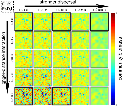
In this paper the authors link between the scales in which processes occur and the scales of the patterns they form, while interacting with scales of environmental effects. They use a LV-like metacommunity model that explicitly includes these scales. A major finding is that while increasing the scale of dispersal homogenizes biodiversity in space, increasing that of interactions creates heterogeneity, emphasizing local patterns. Another key finding is that the aggregated patterns of SAR and BEF cannot capture these differences.
Overall I found the manuscript intriguing. Although I enjoyed reading it, this is not an easy paper to read. It is not necessarily a bad thing, but the authors should be aware that ecologists who are not fluent in theory may not get the message, which is an important one. This can be solved by adding an accessible summary. That said, the problem is clearly presented and well defined. The model fits the questions, and its assumptions are specified. The results are generally well presented. I have a few comments to help improve but nothing too major. I certainly recommend this for PCI ecology.
Comments
Introduction
The statement that it is generally assumed that interactions are local is not completely true. Studies like that of Poisot 2012 in Ecology Lett (and those that have followed), which look at gamma and beta diversity of interactions across patches already treat this problem specifically. Multilayer networks are a next step to this because they explicitly connect (via interlayer edges) the processes that operate between layers of interaction (e.g., interlayer links connecting patches). I do agree though that the issue of interaction scale explicitly and how it interacts with scales of dispersal and environment has not been studied systematically (as far as I know).
Fig. 1: The illustration of the spatial scales in panel A is not clear. Why do arrows range outside the distributions? Maybe a clearer illustration would be to show two species interacting in two patches and other two species interactions in one but not the other? The dispersal is also not clear. Panel C: Not clear what are the yellow and white circles
Model
Environment definition: not clear how V varies in space. What is an environmental scale? Some tangible example would also help here. Also, per L 213: What does a value of E=32 mean? How did you obtain it and what is the range? What is an environment of 320x320? Does that mean that x and y have coordinates 1..320? It would be nice to see a map (landscape) of environmental heterogeneity.
Interactions definitions: How does $\beta$ affect the results? It seems to be a really important variable in defining interaction scale, but there is not sensitivity analysis.
L 188: I is not defined (only later)
For which real-world cases this model is relevant?
Results
Fig 4 and related results: I do not see evidence for the claim that “a large interaction scale I leads to a stronger SAR.” The plots on the local and regional BEF look qualitatively (and almost quantitatively) similar to me. If they are not, this should be shown statistically. The individual runs make the plots messy and do not add meaning. I would leave the mean curves, and maybe, if it is not too hard on the eyes, add shades for CI.
In the SAR, I do not see how “a large interaction scale I leads to a stronger SIR” (Line 339). (what does “stronger” mean?) I do see, however, that when the area is small, the effects of dispersal and interaction scale determine the order of the curves: from the intercept to the inflection point around E, their order corresponds first to the dispersal and then, when dispersal is equal to interaction scale. Therefore, SAR is able to capture scale when I,D<E. What are the “replicates”? This is a deterministic model. So what is the difference between them?
Discussion
Reviewed by anonymous reviewer 1, 22 Nov 2021
The authors have performed a great job trying to link the scales of process and pattern in ecology using a Lotka-Volterra metacommunity model. They point to the importance of the spatial scale of species interactions, previously neglected. Although this may be considered as a simplification of more complex mechanisms, it is a valuable approach as an effective way of taking those into account. Their main finding, that the scale of environmental heterogeneity influences the patterns produced by dispersal and interactions, is relevant nowadays.
This being said, some aspects of the manuscript can be improved. I have the general impression that the manuscript is lengthy and might be more clear, so some editing might help. Also, I have two major comments, both in the discussion, and several minor ones.
Major comments:
l.356-359 This conclusion seems unsuported. You only show results for a single environmental scale (E=32), therefore saying that environmental scale sets the characteristic scale of biodiversity and functioning seems an overstatement. You should show that the SAR does the same for at least one or two more values of E (even though I am sure it would be the case), maybe in the supplementary. Also, I am not sure that functioning, measured with BEF, is set with the environmental heterogeneity alone, as I fail to see from where do you derive this claim.
l.462-465 This is the main weakness of the experiment, using only Lotka-Volterra competitive interactions to extract conclusions applicable to general ecosystems. Other mechanisms may not be well described under L-V dynamics, such as consumer-resource interactions or parasites (see Lafferty et al. 2015 Science), so this weakness should be adressed in the manuscript, maybe in the line of considering L-V dynamics as an effective way of describing this more complex processes.
Minor comments:
Abstract
l. 24 The scaling of species interactions, which may be non-local through mobility, is a relatively new concept that deserve a better explanation. Also, the mention to vectors is not straightforward. Do you mean a vector of environmental states? Or maybe vector species transmitting a disease? Both? The clarity of the phrase in this line should be improved.
l. 28-30 I have trouble dissociating mobility into an interaction component and a dispersal component. Maybe an intuition related to this may be inserted in l.25, consequently improving the interpretation of this result.
l.35-36 Here, I would say that, the scale of environmental heterogeneity influences the scale of the patterns produced by the other processes.
- The abstract ends without much discussion of the results. You don’t address why are these results important.
Intro
l.48-50 I would prefer a more deductive reformulation of the critical question. Given the scale of specific processes, which patterns are possible at different scales? Note that currently the question follows a more abductive reasoning linking the observed pattern to the scale of the processes.
l.54-55 However, at each point in time, interactions are usually local. The concept of interactions at distance is useful as a simplification of complex dynamics implying different processes, in other words, a mean-field approximation to more basic underlying processes.
l.55 Is reference [13] here correct? [13] is a simulation study on heteromyopia… Also I have doubts on l.58
l.58 Salmon returning to their natal streams does not seem an intuitive image for the spatial scale of species interactions (I would frame it in dispersal with some caveats).
l.95-96 This statement is a bit vague. Maybe an example of the kind of biodiversity problems that the study might help solve would convince the reader of the importance of this work.
Methods
l.143-145 I feel that the explanation of species interactions beyond local scales should be introduced before, probably in line 58.
l.210-215 More information is needed here on spectral color and cutoff. Ecologist may not be familiar with these metrics (I am not) and some explanation and references (if available) would be useful, apart from mentioning [33] in the appendix.
l.230-236 Experimental design does not seem clear enough. There are 20 different D&I settings for a given landscape (E=32 for example), called replicates in the methods. However, in figure 4 it seems that each individual D&I settings has more than one replicate (20 in fact). Please clarify how many experiments are performed for each E or D&I setting.
l.259-260 For measuring BEF, why do you choose locations at random when you could sample each location once? Also, do your results change if the regional scale is set differently?
l.267-277 This part would be more accessible including some schematics of what you did in the Appendix.
Results
l.282-297 Little is said about the pattern in Fig. S3, that is contrasting to the one in Fig. 2, and therefore interesting. There, the effect of dispersal is clear at all scales.
l.321 The mention of figure S4a is probably wrong (S5a instead?).
l.324-327 To me, both local and regional BEF look quite similar, just increasing the axis of species richness, so I would modulate these lines.
Discussion
l.413-426 I find that this passage is not very relevant, unless you are able to produce Turing patterns in your setting. I would skip it.
l.427-444 This is an interesting but rather technical discussion that may deserve a place in the Appendix, for the sake of brevity and clarity in the main text.
Reviewed by Gian Marco Palamara, 24 Dec 2021
please see attached PDF
Download the review