
Recommendation
 based on reviews by Kevin Cazelles and 1 anonymous reviewer
How do you estimate the biodiversity of a whole community, or the distribution of abundances and ranges of its species, from presence/absence data in scattered samples?
It all starts with the collector's dilemma: if you double the number of samples, you will not get double the number of species, since you will find many of the same common species, and only a few new rare ones.
This non-additivity has prompted many ecologists to study the Species-Area Relationship. A common theoretical approach has been to connect this spatial pattern to the overall distribution of how common or rare a species can be. At least since Fisher's celebrated log-series [1], ecologists have been trying to, first, infer the shape of the Species Abundance Distribution, and then, use it to predict how many species should be found in a given area or a given number of samples. This has found many applications, from microbial communities to tropical forests, from estimating the number of yet-unknown species to predicting how much biodiversity may be lost if a fraction of the habitat is removed.
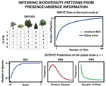
In this elegant work, Tovo et al. [2] propose a method that starts only from presence/absence data over a number of samples, and provides the community's diversity, as well as its abundance and range size distributions. This method is simple, analytically explicit, and accurate: the authors test it on the classic Pasoh and Barro Colorado Island tropical forest datasets, and on simulated data. They make a very laudable effort in both explaining its theoretical underpinnings, and proposing a straightforward step-by-step guide to applying it to data.
The core of Tovo et al's method is a simple property: the scale invariance of the Negative Binomial (NB) distribution. Subsampling from a NB gives another NB, where a single parameter has changed. Therefore, if the Species Abundance Distribution is close enough to some NB (which is flexible enough to accommodate all the data here), we can estimate how this parameter changes when going from (1) a single sample to (2) all the available samples, and from there, extrapolate to (3) the entire community.
This principle was first applied by the authors in a previous study [3] that required abundance data in the samples, rather than just presence/absence. Given that binary occurrence data is far more available in a variety of empirical settings, this extension is worthwhile (including its new predictions on range size distributions), and it deserves to be widely known and tested.
ADDITIONAL COMMENTS
1) To explain the novelty of the authors' contribution, it is useful to look at competing techniques.
Some ""parametric"" approaches try to infer the whole-community Species Abundance Distribution (SAD) by guessing its functional form (Gaussian, power-law, log-series...) and fitting its parameters from sampled data. The issue is that this distribution shape may not remain in the same family as we increase the sampling effort or area, so the regression problem may not be well-defined. This is where the Negative Binomial's scale invariance is useful.
Other ""non-parametric"" approaches have renounced guessing the whole SAD: they simply try to approximate of its tail of rare species, by looking at how many species are found in only one (or a few) samples. From this, they derive an estimate of biodiversity that is agnostic to the rest of the SAD. Tovo et al. [2] show the issue with these approaches: they extrapolate from the properties of individual samples to the whole community, but do not properly account for the bias introduced by the amount of sampling (the intermediate scale (2) in the summary above).
2) The main condition for all such approaches to work is well-mixedness: each sample should be sufficiently like a lot drawn from the same skewed lottery. As long as that condition applies, finding the best approach is a theoretical matter of probabilities and combinatorics that may, in time, be given a definite answer.
The authors also show that ""well-mixed"" is not as restrictive as it sounds: the method works both on real data (which is never perfectly mixed) and on simulations where species are even more spatially clustered than the empirical data. In addition, the Negative Binomial's scale invariance entails that, if it works well enough at some spatial scale, it will also work at all higher scales (until one reaches the edges of the sufficiently-well-mixed community)
3) One may ask: why the Negative Binomial as a Species Abundance Distribution?
If one wishes for some dynamical explanation, the Negative Binomial can be derived from neutral birth and death process with immigration, as shown by the authors in [3]. But to be applied to data, it should only be able to approximate the empirical distribution well enough (at all relevant scales). Depending on one's taste, this type of probabilistic approaches can be interpreted as:
- purely phenomenological, describing only the observational process of sampling from an existing state of affairs, not the ecological processes that gave rise to that state.
- a null model, from which everything in practice is expected to deviate to some extent.
- or a way to capture the statistical forces that tend to induce stable relationships between different patterns (as long as no ecological process opposes them strongly enough).
References
[1] Fisher, R. A., Corbet, A. S., & Williams, C. B. (1943). The relation between the number of species and the number of individuals in a random sample of an animal population. The Journal of Animal Ecology, 42-58. doi: 10.2307/1411
[2] Tovo, A., Formentin, M., Suweis, S., Stivanello, S., Azaele, S., & Maritan, A. (2019). Inferring macro-ecological patterns from local species' occurrences. bioRxiv, 387456, ver. 2 peer-reviewed and recommended by PCI Ecol. doi: 10.1101/387456
[3] Tovo, A., Suweis, S., Formentin, M., Favretti, M., Volkov, I., Banavar, J. R., Azaele, S., & Maritan, A. (2017). Upscaling species richness and abundances in tropical forests. Science Advances, 3(10), e1701438. doi: 10.1126/sciadv.1701438
DOI or URL of the preprint: 10.1101/387456
Version of the preprint: 2
Dear Editor, attached you find our response letter and revised manuscript.
Being the changes only minors, we did not track them in the revised manuscript but they are detailed in the letter.
Thanks and happy new year!
, posted 20 Dec 2018Dear authors,
Thank you for your letter and resubmission, with my sincere apologies for the delays.
Serious concerns have indeed been addressed very satisfactorily, and I would now like to suggest very minor revisions following the comments of one of the reviewers and my own attached. As soon as those are done, I will post my recommendation for the updated preprint.
Besides my annotations of the pdf for typos (attached below), I have a comment on the reviewer's concern about eq 10: it took me a bit to convince myself that this expression is correct and indeed hypergeometric, even if it only takes the canonical form when you replace (M v) by (M M-v) (clearly equal by symmetry) at the top left.
As the interpretation in terms of a hypergeometric distribution is not very intuitive (why would you have n+M-1 balls of which M are successful, and try to get v successes by drawing M-1 balls?), I would recommend instead a small term-by-term explanation: you have (M v) possibilities to choose the v filled bins, (n-1 v-1) possibilities to distribute n balls among v bins so that no bin is empty, and (n+M-1 M-1) ways to distribute n balls in M bins allowing empty bins, then referencing a classic book on combinatorics for these results (e.g. W. Feller's book and its "bars and stars")
Sincerely, Matthieu Barbier
Download recommender's annotations, 17 Dec 2018Dear authors,
This is my second review of your manuscript 'Inferring macro-ecological patterns from local species’ occurrences'. Again, my comments are meant to be constructive, and I hope they will be helpful as you revise your manuscript.
Sincerely,
The authors have taken into account most of my comments and I now have a better understanding of the study. I however think that the manuscript still requires some work, but not much.
In this section, I explain why I think the authors should better explain what a Negative Binomial (NB) on $\mathbb{R}$ is and the link of their approach with the Neutral Theory.
In their revision letter the authors wrote:
"We deem this characterization is somehow misleading for two reasons: i) classically $r \in N$ whereas in our framework $r \in R+$ ii) we recover a negative binomial as the equilibrium distribution of a birth an death process with immigration and we do not see any immediate correspondence between successes and fails of a sequence of binary independent trials and individuals of a species."
Thanks to this comment and the new version of the manuscript I now understand what I missed during the first review. The authors are referring to an extended version of the Negative Binomial (NB extended to $\mathbb{R}$). Given that the 3 references about this distribution provided in the text:
"Our framework exploits the form-invariance property of the Negative Binomial (NB) distribution. Such a distribution emerges as the long time behavior distribution of a birth and death stochastic dynamics, accounting for effective immigration and/or intraspecific interactions [35, 24, 29]." (p.3)
include at least one of the authors of this study, I understand that they are quite familiar with this distribution, but for other ecologists it may not be trivial. Actually I have tried to find other usage of this form of NB and found this link https://stats.stackexchange.com/questions/310676/continuous-generalization-of-the-negative-binomial-distribution that suggests that it is not common but used by a few research groups on bioinformatics [@mccarthydifferential2012]. As it is not a classical distribution (the NB on $\mathbb{N}$ is classical), the authors should highlight this as well as the implications (e.g. the need of a normalizing factor in some equation). This is particularly important because some notations are used in a broader sense, for instance below equation (1), the binomial coefficients used are real number, which implies that the Gamma function is used.
Even more important is to mention the link between this approach and the theoretical work on the Neutral Theory of Biogeography (by these authors and others). This must be explicitly written in the manuscript. I believe that once this explained the authors should drop the justifications pertaining to the need of the absence of spatial correlation (e.g. "Under the hypothesis of absence of spatial correlation" - p.7). This could also be helpful to define the scope of this approach, for instance, p.7:
The proposed method is, under the ‘well mixed’ hypothesis, general and not lim- ited to tropical forests.
I agree, but the authors should rather remind the reader that this approach is limited to systems for which the neutral theory is deemed valid.
The new version of the manuscript better describe what is done but I still had to go through the method section to see the big picture. I think one sentence explaining that the goal of the approach is to use presence/absence data to infer fundamental parameters that will be used to derive RSA, SAC and RSO would be very helpful. The reader must understand at the end of the introduction what is built on the neutral theory and where is the inference part of the method.
Unless I am missing something, equation (10) is wrong. I don't think (10) is a hyper-geometric (it looks like one but it is not). Two options here:
I am totally wrong in which case, the authors need to make this part more accessible: I know what a hypergeometric distribution is but I don't understand why it is relevant here;
I am right so there is something wrong here. Given the definition of $Q_{occ}(v|n,M,1)$, I remain skeptical that a hypergeometric is the best option.
Overall I do not understand the relationship between M and M* (if any).
One important question is whether or not M=A/a. I think the answer is no
but p.7 the authors wrote: "given that the forest can be tiled in M equal-sized cells of area a." which makes me think that it may be yes. Also I think that M=A/a is needed to derive (10) unless $n$ is the total of individuals over A.
I think this question is not properly handled in the current manuscript because it relies on the contrast of two point processes and for the one includin spatial auto-correlation (Thomas), we actually don't know what the clustering values means in term of auto-correlation (is it a lot or not?). I guess one way to address this comment is to progressively increase the clustering values and observe how the errors in Table are affected.
I was wondering whether detection probabilities can be easily integrated in the framework, it may be something to discuss.
p.2 "this method have been" => "this method has been"
p.4 "biodiversity patterns" => "biodiversity relationships"?
Between equations (2) and (3) I would mention that the goal is to have a relationship between the birth and death ratios at two spatial scales ($\xip$ and $\xi{p*}$).
equation (4): what does $\equiv U(p|p^, \xi p^)$ means?
p.7 "This assumption is not essential to our approach" you mean the assumption of equal area, right? This is rather important to compute the RSO, am I wrong?
p.6 I would remind the reader that it needs to use the equation (not numbered) above equation (2) in order to get (7).
McCarthy, Davis J., Yunshun Chen, and Gordon K. Smyth. 2012. “Differential Expression Analysis of Multifactor RNA-Seq Experiments with Respect to Biological Variation.” Nucleic Acids Research 40 (10): 4288–97. https://doi.org/10.1093/nar/gks042.
Download the reviewThe authors have significantly improved the presentation, which is now clear and engaging. They have also addressed my other comments.
I now warmly support recommending this paper in PCI Ecology.
DOI or URL of the preprint: 10.1101/387456
Version of the preprint: 1
, posted 12 Nov 2018Dear Authors,
I agree with both reviewers that the work in manuscript is truly worthy of recommendation, but would deserve a clearer presentation to really get the attention it deserves.
In addition to the two reviews, a third colleague (anonymously) noted that this work is very relevant and interesting, but that there should be no shortcuts taken in the writing. Some basic assumptions are not explained (e.g. why take the negative binomial? we can come up with a justification, but it should be explicit already). Most importantly, the model description is very sloppy with incomplete definitions and inconsistent use of variables and parameters. The introduction could be more explicit about the concepts it refers to.
Maybe part of this is tied to the possible redundancy with a prior work, as noted in the review of K Cazelles, in which case I concur that the authors should make a clear-cut choice, making this manuscript either an explicit follow-up (so that the reader knows where to go for details), or something much more pedagogical that can encourage other scientists to use this method.
I think it is good practice for authors to try to read the paper through the eyes of someone who never encountered any of these methods or questions, and try to judge whether, when a concept appears, there is sufficient information to either understand it on the spot or know how to learn more about it (if the concept is relevant to the results, the answer to that should be "later in the text", rather than "somewhere in another reference", unless it is very clear from the start that this manuscript is a follow-up to one specific other work).
Detailed comments:
-"these latter methods make no assumption on the RSA distribution and they thus perform no fit of empirical patterns, rather they only take into account rare species, which are intuitively assumed to carry all the needed information on the undetected species in a sample" After reading this sentence, I have honestly no idea how nonparametric models work, and what it means for them to "perform no fit of empirical patterns". Can you try being a bit more descriptive? (without necessarily being much longer, just less oblique) (NB: After reading further down, I now understand what is happening here, but I don't think I could have understood it from this sentence; maybe give a short account of how parametric and nonparametric methods work in general, whether the former traditionally use part of the test data to do the fitting or whether they use different patterns for fit and prediction as you do, etc.)
Is Table 2 simply missing its caption, or was it planned not to have one? If you add one with the definition of all the terms that are not defined in there (C, etc.), it would help quite a bit. The caption may also be where you put some explanations of the nonparametric methods, if you think they would clutter the introduction.
"derived as the steady-state RSA of a birth and death stochastic dynamics, accounting for effective immigration and/or intraspecific interactions" It would be worthwhile having a short (even 1 sentence) explanation of how this works. In particular, it seems important for the reader to understand how much of what you say is based on purely statistical effects versus how much relies on specific biological assumptions.
"We denote as P (n|1) the relative species abundance, – i.e. the probability that a species has exactly n individuals" I'm confused as to how this is a relative species abundance
"with parameters (r, ξ) (r is known as the clustering coefficient)" Please give any intuition of what parameters r and xi mean (where they come from qualitatively in the derivation in your previous work, and how they shape the distribution)
"In order to reduce the number of parameters to fit from three to two (see (7))" I don't see what the third parameter is in (8), it seems you have only (r, ξp∗ )
"we rescale the setting, by assuming that the global scale p = 1 is actually the one where we have data, i.e. the sampling scale p∗ = na/A."
I think this sentence is very confusing since it says that << "p=1" == "p∗ = na/A" >> which makes little mathematical sense. After some parsing I understood something like: "we now want to make predictions of what happens when subsampling the data, instead of using the data as a subsample of the unknown true distribution. For this specific use, we define the total area A' as A'=na given we have n measurements, each of area a". However, this is not the same "a" as used in page 4 (where "a" was, in a sense, the total sampled area A') so this is confusing. Also, when has n become a number of measurements? Are you saying that each area a must now contain exactly one individual? If so, you should really note that beforehand.
Please add at least this level of detail and clarity if that was indeed your meaning. The notion that we are using the same formulas in different ways to subsample for fitting and to extrapolate from the fit is very interesting, but it is tricky and should be made crystal clear.
"we compute the empirical average of the species observed in all subsets of k cells." of the number of species
"and compute the C × S presence/absence matrix," C switches between being a set and being the cardinal of that set; maybe redefine C here (and potentially change notation for the set)
"In the case of the NB forest, the two methods performed very well for both the random and the clumped distribution with an average prediction error below 1% in absolute value (see Table1). In the Thomas distributed forests, the error increased,"
Do you mean the LN forests in that last sentence? The Thomas distributed forests = the clumped distribution mentioned in the previous sentence
Typos:
p2: at a that spatial scale
p3: however our method can applied
p5: helps us linking => link
p7: ωsi = 1 if species i => species s
, 07 Sep 2018Dear authors,
This is my review of your manuscript Report on 'Inferring macro-ecological patterns from local species’ occurrences'. My comments are meant to be constructive, and I hope they will be helpful as you revise your manuscript. Note that I used markdown to write this review so you will find some tags in the text below. For the sake of clarity (especially for equations), I have attached a pdf version of my review.
Sincerely,
In this manuscript Anna Tovo and colleagues propose a statistical framework that allows the inference of several biodiversity patterns based on the matrix of presence-absence matrix, the assumption that the Relative Species Abundance (RSA) follows a Negative-Binomial (NB) distribution and the absence of strong spatial correlations among the set of species considered. The manuscript is overall clear, well-structured and deals with a topic that could interest many ecologists as it proposes to derive valuable information based on the widely used presence-absence matrices.
Despite the quality of the manuscript, I believe that this manuscript requires some work to be recommended by PCI Ecology. In particular, the authors must put substantial efforts into the methods section in order to 1- better explain how the framework work, 2- better emphasize the difference between this manuscript their previous study [@tovoupscaling2017] and 3- to discuss the scope of their approach. In the following lines, I did my best to detail my concerns regarding these points.
As mentioned above, this paper may interest many ecologists given its topic. I however think that the current version of the manuscript may appear quite impenetrable for many of them due to the lack of explanations of some mathematical concepts and notations in the methods section. Below I provide several suggestions to improve the clarity of this section.
I think it would be very helpful to remember what a Negative Binomial distribution is. A single sentence would be sufficient, something along this: "in a succession of Bernouilli trials in which the success probability is $\xi$, the negative binomial distribution of parameter $(r, \xi)$ models the probabilities associated to the number of trials required to obtain exactly $r$ successes."
Throughout the methods section, the authors use $P$ and $\mathcal{P}$. To me, this is quite confusing as according to the text they both are probabilities, so why using these notations?
Point 2 is also confusing because it seems like $P(n|1)$ is actually not a probability. Indeed $\mathcal{P}(n|r,\xi)$ is a negative binomial, so
$$\sum^{+\infty}_n \mathcal{P}(n|r,\xi) = 1$$
But then,
$$\sum^{+\infty}_n P(n|1) = c(r,\xi)$$
so, "the probability that a species has exactly n individuals – at the whole forest scale" do not sum to 1, what am I missing here? Why another "NB normalization" is needed? There is a explanation of this in [@tovoupscaling2017] but it should be clarify here.
"[...], the conditional probability that a species has k individuals in the smaller area a = pA, given that it has total abundance n in the whole forest of area A is given by the binomial distribution" (p.4). If I am correct, I would explain here that the assumption of spatial correlation is important to use the binomial distribution here.
Why do the authors use $\widehat{\xip}$ rather than $\widehat{\xip}$? Is it because it is an estimator? This should be clarified. In the same vein, $\equiv U(p|p^* , \widehat{\xi}_{p^* } )$ in equation (4) may prevent readers from understanding the demonstration, this should be commented with words.
I think it would have been clearer to state: "S_p(k) denotes the number of species having k individuals at the scale p" which is directly applicable for $p^* $.
"[...], by assuming that the global scale p = 1 is actually the one where we have data, [...]." (p.6). I think the authors should develop what this means practically.
"Under the mean field hypothesis, [...]" (p.6). The authors should remind the readers what this means.
"In words: for every scale pk, we compute the empirical average of the species observed in all subsets of k cells." (p.8). How the authors deal with this from a numerical standpoint, because, for instance, choosing 100 cells among 98x98, represent more than $10^{240}$ possibilities, what did I miss?
There are a high degree of similarity between what is done here and what the authors did in [@tovoupscaling2017]. The goal are the same, the method is here applied on two data sets included in the previous studies and many equations are identical. Moreover the reader should refer to this previous study to fully understand the demonstration. I think it is very important that the authors better explain what has been done in their previous study and what brings this new manuscript.
My feeling is that the authors have two options. The first is, to restrict their manuscript to its novelty. What I mean here is that the authors could build on the top of [@tovoupscaling2017] without repeating the equations they have already published and make it very clear what they did at the beginning of the section and then highlight the new developments. In the current version, there are scattered sentences about the previous study but I am still wondering to what extent this study is new. For instance, p.14, the authors wrote: "Our framework not only provides a generalization of the method recently proposed in [29], [...] but I do not see the generalization in this paper. The second option is a very didactic paper to better guide readers through the framework and convince them to use it. This is the one I would recommend and I think the advice I provided above may be useful in this respect. In this didactic piece, I would suggest to add a few sentences about the numerical implementation of it, starting by mentioning where to find it.
The authors must discuss the scope of their framework thoroughly. In the current version of the manuscript, the authors have applied their framework on simulated forests and two tropical forests. So a first question: is this method only designed for tree species in tropical forest? I guess no, otherwose they would not have present their method as a general one in the abstract. I however question its generality, especially given that I think the detectability of the species is crucial to apply this method, am I right? This would explain why tree species are well-suited to exemplify the method. I believe this is a first point to be added when discussing the scope of the method. A second is linked with the assumption introduces page 4:
"Assuming that the local RSA is not affected by spatial correlations due to both inter-specific and intra-specific interactions and strong environmental gradients [...]."
To me, this should be further developed. For instance, how this could be tested? I think the authors should further stress that the assumptions made regard the relationships at the scale of the set of species, not the individuals species and then discuss what group of species is likely to meet the assumptions.
p.1 (abstract, point 3): "This framework, derived from first principles on the basis of biological processes[...]", I do not understand why this framework is "derived from first principles on the basis of biological processes".
p.1 "[...] as well as a new emergent pattern, which is the Relative Species Occupancy (RSO)." The authors introduced and used the RSO throughout their manuscrit. I do not understand why the authors introduces it, is it more than a prediction of their framework that can be tested? If so, I would discuss the potential applications of the RSO in ecology.
p.2 I would add a little more context about the RSA. In particular, I would introduce another RSA, the zero-sum multinomial that was convincingly applied by Hubbel on tropical trees in its classical Neutral Theory of Biogeography [@hubbellunified2001].
Figure 2: Is the flat line for the Data something expected?
Table 2: All notations used must be defined. So, C should be defined in the table. Also, I would write "number" rather than using "#" and add a column references to associate an estimator with at least one paper.
p.12: "We provide an open source R code that perform" a "s" is missing.
Hubbell, Stephen P. 2001. The Unified Neutral Theory of Biodiversity and Biogeography. Monographs in Population Biology 32. Princeton: Princeton University Press. Tovo, Anna, Samir Suweis, Marco Formentin, Marco Favretti, Igor Volkov, Jayanth R. Banavar, Sandro Azaele, and Amos Maritan. 2017. “Upscaling Species Richness and Abundances in Tropical Forests.” Science Advances 3 (10): e1701438. https://doi.org/10.1126/sciadv.1701438.
Download the reviewThe authors describe a method to predict the species richness and other biodiversity patterns, using presence-absence data on smaller surveyed plots. The method relies on a biologically-based model for how these properties vary with the spatial scale. I found the basic idea interesting and sound. The comparison with other methods to predict the richness in forest data (Fig. 2), makes a convincing case for the merits of the proposed method. The new pattern suggested by the authors, RSO, and the fat tails it displays, are interesting and seem worthy of further exploration (in future works).
A number of comments: -- In Fig. 3, the panels showing RSA and RSO data make it hard to judge the level of agreement between prediction and data. This is important in light of the authors claim that "all three patterns are well described by our framework". In particular, most of the values in those panels are concentrated at low frequencies, where the theoretical line is almost as wide as the bin height. These panels would benefit from logarithmic vertical-axis. In addition, in order to compare the tail of the distribution (claimed to be fat for the RSO), where many of the bins are empty, a plot of the sorted values versus the cumulative distributions would be helpful.
-- Fig. 2: Do the authors understand why the final richness is consistently underestimated, is there a reason for this bias?
-- Regarding the derivation in Section 1.1. The derivation is very clear, down to about Eq. (5). Then I felt it became less clear. First, until Eq. (5,6) the text considers the probabilities of abundances, so the richness S* at a given scale is also a distribution. But then, unannounced, Eq. (5,6) treat S* as fixed numbers. Are these the means of S? Is it always the case that the distribution is narrow (are S always large enough)? This should be made explicit. After Eq. (8) things become confusing. What are the "three parameters" that are reduced to two? What does it mean that "p=1 is actually the scale where we have the data"? In the equation "p=na/A", is "n" the number of cells (before "n" was the number of individuals)? A little below, "M" is used for the number of cells, what is the difference? And in page 7, top, p is again only a fraction of the total area. These parts would benefit from more consistent notation, defined upfront, and some clearing up of the derivation.
-- In Eq. (12) the spatial information -- which cells are neighbors, etc. -- is thrown away. It would be helpful to note this at this point in the manuscript.
